Martingale Resampling Applications in Survival Analysis

knitr::opts_chunk$set(
  echo = TRUE, 
  message = FALSE, 
  warning = FALSE,
  fig.width = 10, 
  fig.height = 6
)
options(warn = -1)
library(survival)
library(ggplot2)
library(weightedsurv)

Introduction

Martingale resampling (perturbation resampling) provides a powerful and flexible approach to inference in survival analysis. While asymptotic distributions are available for many common analysis methods, resampling-based inference

May have greater accuracy in small samples, and
Extends to complex processes where asymptotics are not readily available (Dobler, Beyersmann, and Pauly 2017).

This vignette demonstrates martingale resampling applications in the weightedsurv package using two breast cancer datasets:

GBSG — a randomized clinical trial evaluating hormonal therapy (Schumacher et al. 1994).
Rotterdam — an observational study where propensity-score weighting is used to adjust for confounding (Royston and Altman 2013).

The examples include:

Simultaneous confidence bands for survival (KM) arm differences
Cumulative RMST curves with pointwise and simultaneous bands across follow-up (Zhao et al. 2016)
Weighted analyses using propensity-score (IPTW) weights

Brief Review of Counting Processes

We observe $(X_{i,j}, \Delta_{i,j}, Z_{i,j})$ where for subjects in group $j$ ( $Z_i = j$ ):

$X_i = \min(T_i, C_i)$ and $\Delta_i = I(T_i \leq C_i)$
The at-risk process: $Y_{i,j}(t) = I(X_i \geq t, Z_i = j)$
The counting process: $N_{i,j}(t) = I(X_i \leq t, \Delta_i = 1, Z_i = j)$

The aggregate counting processes $\bar{N}_j(t) = \sum_{i=1}^{n_j} N_{i,j}(t)$ count the observed events through time $t$ for the control ( $j=0$ ) and experimental ( $j=1$ ) arms.

The Weighted Log-Rank Test

The weighted log-rank (WLR) statistic of class $K^{+}$ is

$W_K = \int_0^{\infty} \left\{ \frac{K(t)}{\bar{Y}_0(t)} d\bar{N}_0(t) - \frac{K(t)}{\bar{Y}_1(t)} d\bar{N}_1(t) \right\} = \int_0^{\infty} K(t)\, d\left\{\hat\Lambda_0(t) - \hat\Lambda_1(t)\right\},$

where $K(t) = \sqrt{\frac{n_0 + n_1}{n_0 n_1}}\, w(t)\, \frac{\bar{Y}_0(t)\, \bar{Y}_1(t)}{\bar{Y}_0(t) + \bar{Y}_1(t)}$ with Fleming–Harrington weights $w(t) = [\hat{\bar{F}}(t^{-})]^{\rho}[1 - \hat{\bar{F}}(t^{-})]^{\gamma}$ , $\rho \geq 0$ , $\gamma \geq 0$ .

Martingale Representation

Under the null, $W_K$ can be written as a sum of martingale integrals:

$W_K = \sum_{i=1}^{n_0} \int_0^{\infty} \frac{K(t)}{\bar{Y}_0(t)}\, dN_{i,0}(t) - \sum_{i=1}^{n_1} \int_0^{\infty} \frac{K(t)}{\bar{Y}_1(t)}\, dN_{i,1}(t),$

where the $N_{i,j}(t)$ ’s can be replaced by the corresponding martingales $M_{i,j}(t) = N_{i,j}(t) - \int_0^t Y_{i,j}(s)\lambda_j(s)\,ds$ under the null.

Resampling Recipe

The resampled statistic $W^{\dagger}$ is constructed as:

$W^{\dagger} = \sum_{i=1}^{n_0} \int_0^{\infty} \left\{\frac{K(t)}{\bar{Y}_0(t)}\, dN_{i,0}(t)\right\} G_{i,0} - \sum_{i=1}^{n_1} \int_0^{\infty} \left\{\frac{K(t)}{\bar{Y}_1(t)}\, dN_{i,1}(t)\right\} G_{i,1},$

where $G_{i,j}$ are $n$ i.i.d. $N(0,1)$ random variables. The martingale increments $dM_{i,j}$ are represented by independent standard normal random variables (independent of the data) that are multiplied by the observable counting process increments $dN_{i,j}$ , with unknown parameters estimated by consistent estimators (Dobler, Beyersmann, and Pauly 2017).

GBSG Trial Data: Unweighted Analysis

Data Preparation

We use the GBSG randomized trial data from the survival package, converting follow-up from days to months.

df_gbsg <- gbsg
df_gbsg$tte <- df_gbsg$rfstime / 30.4375
df_gbsg$event <- df_gbsg$status
df_gbsg$treat <- df_gbsg$hormon
df_gbsg$grade3 <- ifelse(df_gbsg$grade == "3", 1, 0)

tte.name <- "tte"
event.name <- "event"
treat.name <- "treat"
arms <- c("treat", "control")

Counting Process Summary and Log-Rank Test

The df_counting() function prepares the survival data in counting-process format and computes the standard log-rank test (Fleming–Harrington $\rho=0, \gamma=0$ ), weighted log-rank statistics, and Cox model results.

dfcount_gbsg <- df_counting(
  df = df_gbsg, 
  tte.name = tte.name, 
  event.name = event.name, 
  treat.name = treat.name, 
  arms = arms, 
  by.risk = 12, 
  scheme = "fh", 
  scheme_params = list(rho = 0, gamma = 0), 
  lr.digits = 4, 
  cox.digits = 3
)

Kaplan-Meier Curves

plot_weighted_km(
  dfcount = dfcount_gbsg, 
  conf.int = TRUE, 
  show.logrank = TRUE, 
  ymax = 1.05, 
  xmed.fraction = 0.725
)
title(main = "GBSG (trial) data: unweighted")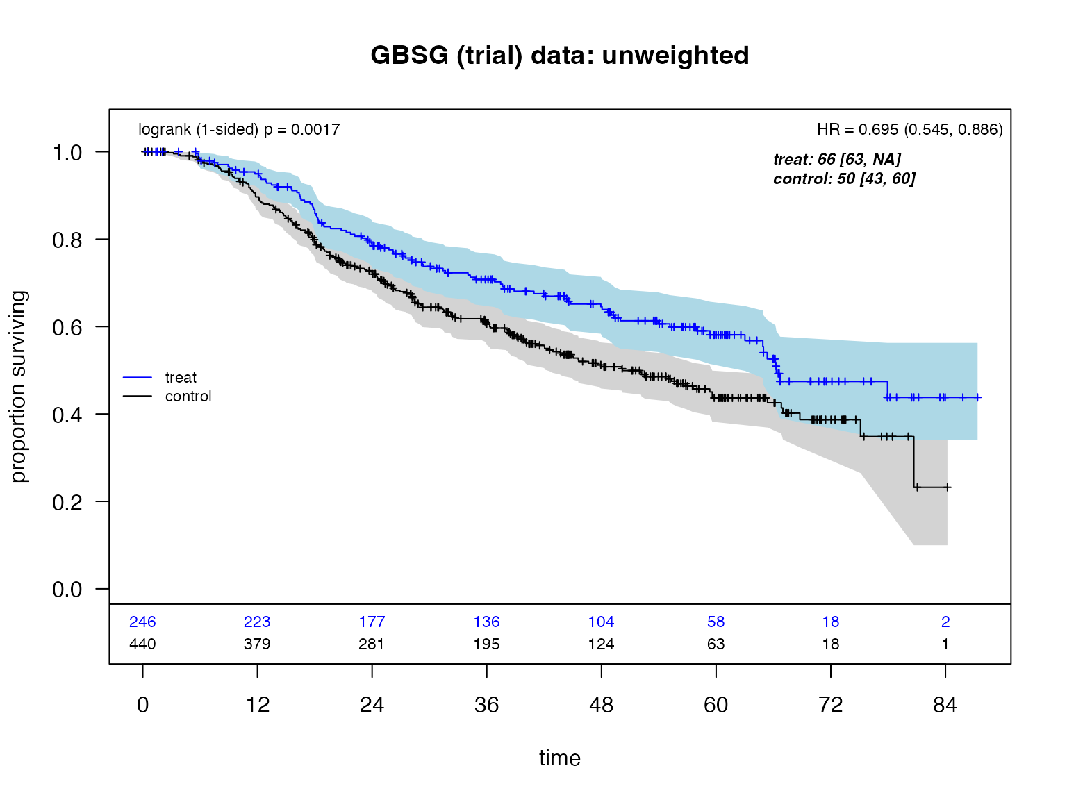

Rotterdam Observational Data: Propensity-Score Weighted Analysis

Data Preparation and Propensity Score Estimation

The Rotterdam dataset is observational, so we use inverse probability of treatment weighting (IPTW) with stabilized propensity-score weights to adjust for confounding.

gbsg_validate <- within(rotterdam, {
  rfstime <- ifelse(recur == 1, rtime, dtime)
  t_months <- rfstime / 30.4375
  time_months <- t_months
  status <- pmax(recur, death)
  ignore <- (recur == 0 & death == 1 & rtime < dtime)
  status2 <- ifelse(recur == 1 | ignore, recur, death)
  rfstime2 <- ifelse(recur == 1 | ignore, rtime, dtime)
  time_months2 <- rfstime2 / 30.4375
  grade3 <- ifelse(grade == "3", 1, 0)
  treat <- hormon
  event <- status2
  tte <- time_months
  id <- as.numeric(1:nrow(rotterdam))
  SG0 <- ifelse(er <= 0, 0, 1)
})

df_rotterdam <- subset(gbsg_validate, nodes > 0)

We fit a propensity score model and compute stabilized IPTW weights:

fit.ps <- glm(
  treat ~ age + meno + size + grade3 + nodes + pgr + chemo + er, 
  data = df_rotterdam, 
  family = "binomial"
)

pihat <- fit.ps$fitted
pihat.null <- glm(treat ~ 1, family = "binomial", data = df_rotterdam)$fitted

wt.1 <- pihat.null / pihat
wt.0 <- (1 - pihat.null) / (1 - pihat)
df_rotterdam$sw.weights <- ifelse(df_rotterdam$treat == 1, wt.1, wt.0)

# Truncated weights (winsorized at 5th/95th percentiles)
df_rotterdam$sw.weights_trunc <- with(df_rotterdam, 
  pmin(pmax(sw.weights, quantile(sw.weights, 0.05)), quantile(sw.weights, 0.95))
)

Unweighted vs. Weighted KM Curves

dfcount_rotterdam_unwtd <- df_counting(
  df = df_rotterdam, 
  tte.name = tte.name, 
  event.name = event.name, 
  treat.name = treat.name, 
  arms = arms, 
  by.risk = 36, 
  risk.add = -50
)

dfcount_rotterdam_wtd <- df_counting(
  df = df_rotterdam, 
  tte.name = tte.name, 
  event.name = event.name, 
  treat.name = treat.name, 
  arms = arms, 
  by.risk = 36, 
  risk.add = -50, 
  weight.name = "sw.weights"
)

par(mfrow = c(1, 2))
plot_weighted_km(
  dfcount = dfcount_rotterdam_unwtd, 
  xmed.fraction = 0.4, 
  arm.cex = 0.475, 
  risk.cex = 0.45, 
  risk_offset = 0.125
)
title(main = "Unweighted K-M curves")

plot_weighted_km(
  dfcount = dfcount_rotterdam_wtd, 
  xmed.fraction = 0.4, 
  arm.cex = 0.475, 
  risk.cex = 0.45, 
  risk_offset = 0.125
)
title(main = "Weighted K-M curves (stabilized PS)")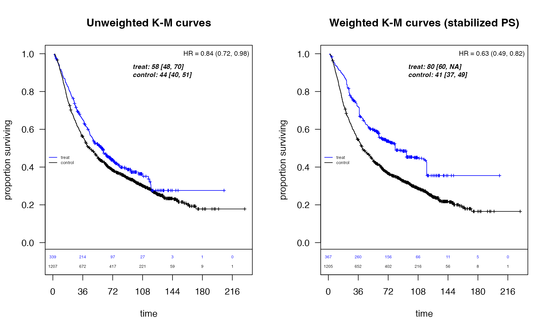

Comparison: GBSG Trial vs. Rotterdam PS-Weighted

par(mfrow = c(1, 2))
plot_weighted_km(
  dfcount = dfcount_gbsg, 
  conf.int = TRUE, 
  xmed.fraction = 0.4, 
  ymax = 1.05, 
  arm.cex = 0.475, 
  risk.cex = 0.45
)
title(main = "GBSG (trial) unweighted")

plot_weighted_km(
  dfcount = dfcount_rotterdam_wtd, 
  conf.int = TRUE, 
  xmed.fraction = 0.4, 
  arm.cex = 0.475, 
  risk.cex = 0.45
)
title(main = "Rotterdam PS-weighted")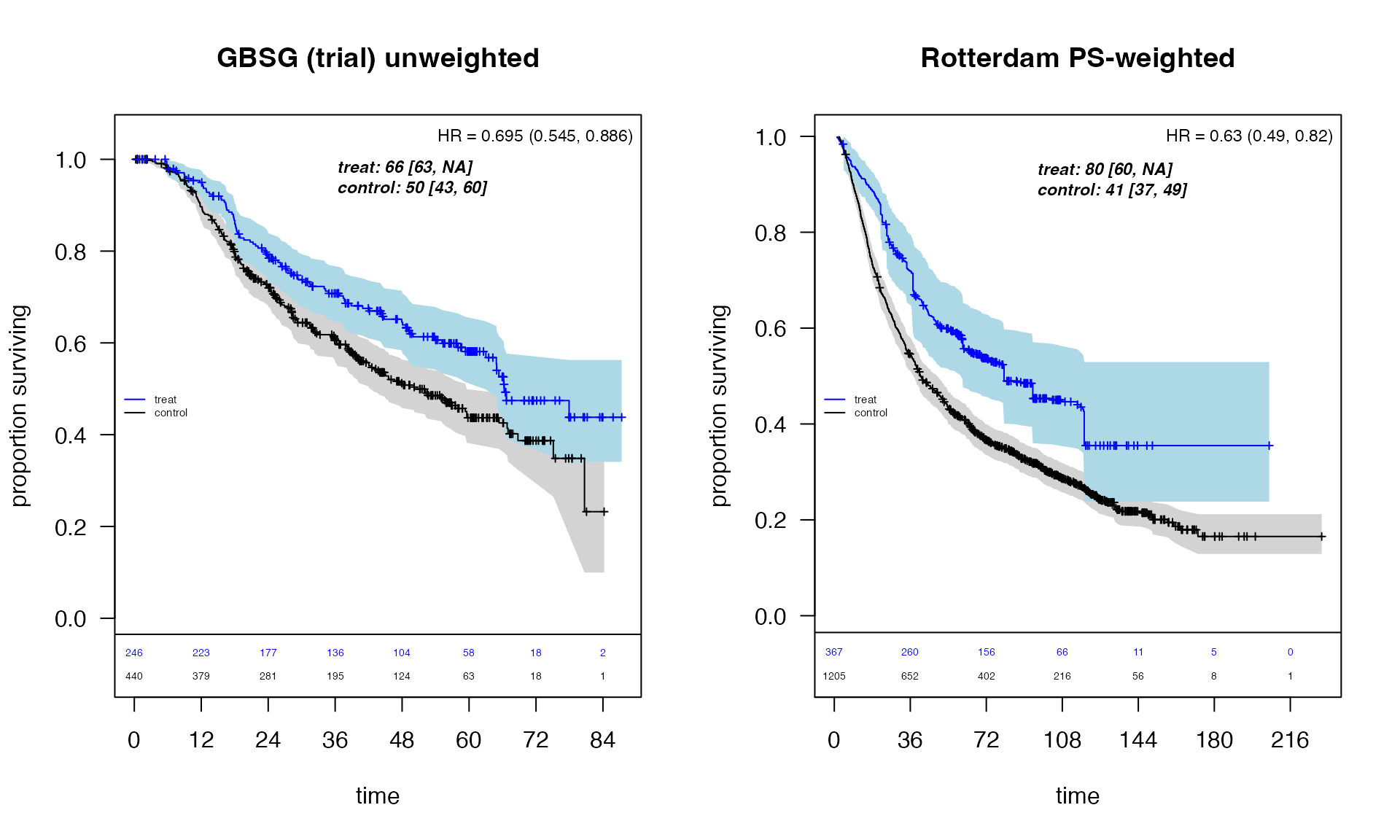

The propensity-score weighted Rotterdam analysis shows a treatment effect pattern broadly consistent with the randomized GBSG trial, supporting the validity of the observational comparison after confounding adjustment.

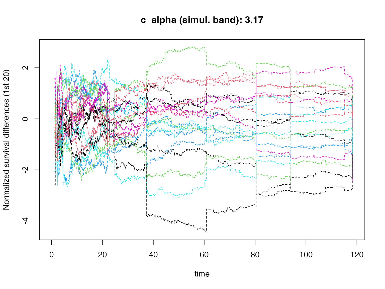
Simultaneous Confidence Bands for Survival Differences

Rotterdam Weighted Survival Difference Bands

The plotKM.band_subgroups() function computes KM survival difference estimates along with pointwise and simultaneous confidence bands using martingale resampling. The simultaneous band provides uniform coverage:

$P\left(\sup_{t \leq \tau} \left|(\widehat{S}_1 - \widehat{S}_0)(t) - (S_1 - S_0)(t)\right| \leq c_{\alpha}\right) \approx 1 - \alpha.$

par(mfrow = c(1, 1))
temp_rotterdam <- plotKM.band_subgroups(
  df = df_rotterdam,
  xlabel = "Months", 
  ylabel = "Survival difference",
  yseq_length = 5, 
  cex_Yaxis = 0.7, 
  risk_cex = 0.7,
  tau_add = 42, 
  by.risk = 24, 
  risk_delta = 0.075, 
  risk.pad = 0.03, 
  ymax.pad = 0.125,
  tte.name = tte.name, 
  treat.name = treat.name, 
  event.name = event.name, 
  weight.name = "sw.weights",
  draws.band = 1000, 
  qtau = 0.025, 
  show_resamples = TRUE
)

legend("topleft", 
  c("Difference estimate", "95% pointwise CIs"),
  lwd = c(2, 1), col = c("black"), lty = c(1, 2), bty = "n", cex = 0.7
)
title(main = "Rotterdam PS-weighted survival differences")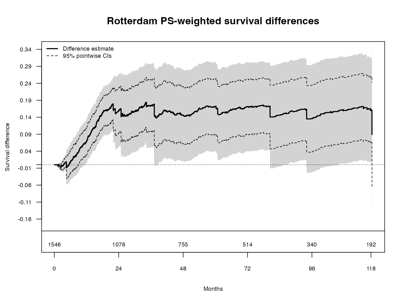

The grey traces show individual resampled processes ( $W^{\dagger}$ ), illustrating the perturbation-resampling distribution from which the simultaneous band critical value is computed.

Cumulative RMST Curves Across Follow-Up

Combined Analysis: Trial and Observational Data

The restricted mean survival time (RMST) at time $\tau$ is defined as $\mu(\tau) = \int_0^{\tau} S(t)\,dt$ , the area under the survival curve up to $\tau$ . Rather than evaluating RMST at a single time point, we study the cumulative RMST curve $\tau \mapsto \hat\mu_1(\tau) - \hat\mu_0(\tau)$ across the entire follow-up period.

Simultaneous confidence bands for the RMST difference curve are constructed via martingale resampling, providing uniform coverage over the range of $\tau$ values (Zhao et al. 2016).

The cumulative_rmst_bands() function takes the fitted object from plotKM.band_subgroups() and computes the cumulative RMST curves with both pointwise and simultaneous bands:

draws <- 1000
par(mfrow = c(2, 2))

# --- GBSG: KM difference bands ---
temp_gbsg <- plotKM.band_subgroups(
  df = df_gbsg, 
  Maxtau = NULL,
  xlabel = "Months", 
  ylabel = "Survival difference",
  yseq_length = 5, 
  cex_Yaxis = 0.7, 
  risk_cex = 0.7,
  by.risk = 6, 
  risk_delta = 0.075, 
  risk.pad = 0.03,
  tte.name = tte.name, 
  treat.name = treat.name, 
  event.name = event.name, 
  draws.band = draws, 
  qtau = 0.025, 
  show_resamples = FALSE
)
legend("topleft", 
  c("Difference estimate", "95% pointwise CIs"),
  lwd = c(2, 1), col = c("black"), lty = c(1, 2), bty = "n", cex = 0.75
)
title(main = "GBSG: KM survival differences")

# --- GBSG: Cumulative RMST bands ---
get_bands_gbsg <- cumulative_rmst_bands(
  df = df_gbsg, 
  fit = temp_gbsg$fit_itt, 
  tte.name = tte.name, 
  event.name = event.name, 
  treat.name = treat.name, 
  draws_sb = draws, 
  xlab = "months", 
  rmst_max_cex = 0.75
)
legend("topleft", 
  c("Cumulative RMST estimate", "95% pointwise CIs"),
  lwd = c(2, 1), col = c("black"), lty = c(1, 2), bty = "n", cex = 0.75
)

# --- Rotterdam weighted: KM difference bands ---
temp_rotterdam2 <- plotKM.band_subgroups(
  df = df_rotterdam,
  xlabel = "Months", 
  ylabel = "Survival difference",
  yseq_length = 5, 
  cex_Yaxis = 0.7, 
  risk_cex = 0.7,
  tau_add = 42, 
  by.risk = 12, 
  risk_delta = 0.075, 
  risk.pad = 0.03, 
  ymax.pad = 0.125,
  tte.name = tte.name, 
  treat.name = treat.name, 
  event.name = event.name, 
  weight.name = "sw.weights",
  draws.band = draws, 
  qtau = 0.025, 
  show_resamples = FALSE
)
legend("topleft", 
  c("Difference estimate", "95% pointwise CIs"),
  lwd = c(2, 1), col = c("black"), lty = c(1, 2), bty = "n", cex = 0.7
)
title(main = "Rotterdam PS-weighted: KM differences")

# --- Rotterdam weighted: Cumulative RMST bands ---
get_bands_rotterdam <- cumulative_rmst_bands(
  df = df_rotterdam, 
  fit = temp_rotterdam2$fit_itt, 
  tte.name = tte.name, 
  event.name = event.name, 
  treat.name = treat.name, 
  weight.name = "sw.weights", 
  draws_sb = draws, 
  xlab = "months", 
  rmst_max_cex = 0.7
)
legend("topleft", 
  c("Cumulative RMST estimate", "95% pointwise CIs"),
  lwd = c(2, 1), col = c("black"), lty = c(1, 2), bty = "n", cex = 0.7
)

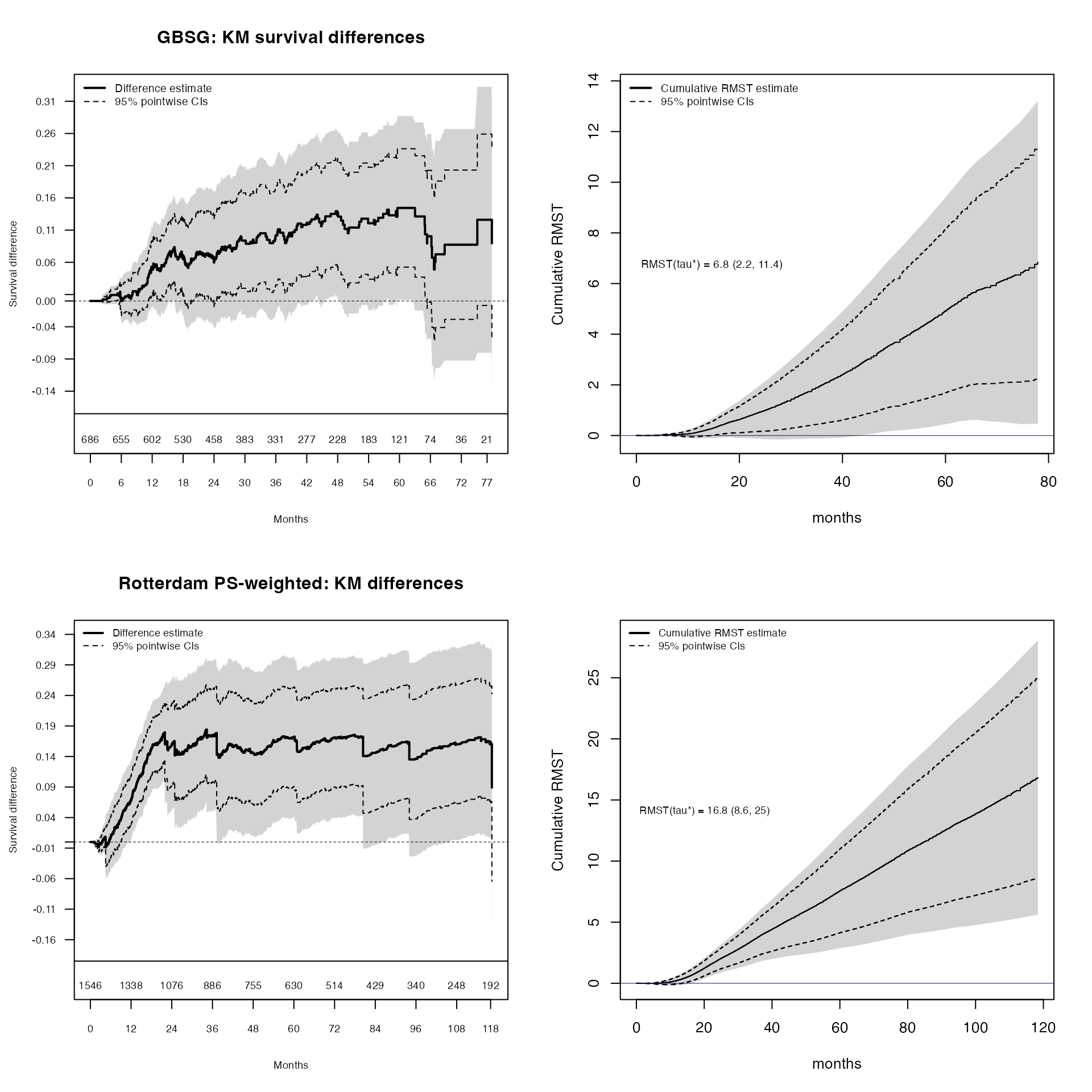
Top row (GBSG trial): The KM survival difference (left) shows the instantaneous treatment gap at each time point, while the cumulative RMST difference (right) shows the accumulated treatment benefit in months gained. The RMST curve integrates the KM difference, providing a clinically interpretable time-scale summary.

Bottom row (Rotterdam weighted): The same pair of analyses using propensity-score weighted estimation from the observational Rotterdam data. The weighted RMST curve shows a cumulative treatment benefit that grows steadily over follow-up, consistent with the GBSG trial findings.

Workflow Summary

The typical workflow for martingale resampling analyses in weightedsurv follows two key steps.

Step 1: KM difference bands. Call plotKM.band_subgroups() to estimate survival differences and compute simultaneous confidence bands. This function returns a fitted object containing the KM estimates and resampling results.

Step 2: Cumulative RMST bands. Pass the fitted object from Step 1 to cumulative_rmst_bands(), which computes the cumulative RMST difference curve and its simultaneous bands using the same fitted survival estimates.

For weighted analyses (e.g., propensity-score adjustment), both functions accept a weight.name argument specifying the column of subject-specific weights in the data frame. The resampling distribution is modified accordingly, with the at-risk process $\bar{Y}_j(t)$ replaced by the weighted version $\bar{Y}_j^w(t) = \sum_i w_i Y_{i,j}(t)$ .

# Step 1: KM survival difference with simultaneous bands
fit <- plotKM.band_subgroups(
  df = mydata,
  tte.name = "tte", treat.name = "treat", event.name = "event",
  weight.name = "ps_weights",   # optional: for weighted analysis

  draws.band = 1000
)

# Step 2: Cumulative RMST bands (uses fit from Step 1)
rmst_result <- cumulative_rmst_bands(
  df = mydata, 
  fit = fit$fit_itt,
  tte.name = "tte", event.name = "event", treat.name = "treat",
  weight.name = "ps_weights",   # must match Step 1
  draws_sb = 1000
)

Summary

This vignette illustrated how martingale resampling provides flexible, nonparametric inference for survival analysis. Key advantages of this approach include:

Simultaneous coverage: Confidence bands maintain nominal coverage uniformly across all time points, unlike pointwise intervals.
Model-free: No proportional hazards or other parametric assumptions are required.
Weighted extension: The same resampling framework applies naturally to propensity-score weighted analyses of observational data.
Complementary perspectives: KM survival differences capture the instantaneous treatment gap, while cumulative RMST differences summarize the cumulative treatment benefit in clinically interpretable units (months gained).

The weightedsurv package implements these methods via plotKM.band_subgroups() for KM difference bands and cumulative_rmst_bands() for RMST curves, with a shared workflow that ensures consistency between the two analyses.

References

Dobler, D., J. Beyersmann, and M. Pauly. 2017. “Non-Strange Weird Resampling for Complex Survival Data.” Biometrika 104 (3): 699–711.

Royston, Patrick, and Douglas G. Altman. 2013. “External Validation of a Cox Prognostic Model: Principles and Methods.” BMC Medical Research Methodology 13: 33. https://doi.org/10.1186/1471-2288-13-33.

Schumacher, M, G Bastert, H Bojar, K Hübner, M Olschewski, W Sauerbrei, C Schmoor, C Beyerle, R L Neumann, and H F Rauschecker. 1994. “Randomized 2 x 2 Trial Evaluating Hormonal Treatment and the Duration of Chemotherapy in Node-Positive Breast Cancer Patients. German Breast Cancer Study Group.” Journal of Clinical Oncology 12 (10): 2086–93. https://doi.org/10.1200/JCO.1994.12.10.2086.

Zhao, Lihui, Brian Claggett, Lu Tian, Hajime Uno, Marc A. Pfeffer, Scott D. Solomon, Lorenzo Trippa, and L. J. Wei. 2016. “On the Restricted Mean Survival Time Curve in Survival Analysis.” Biometrics 72 (1): 215–21.

Larry Leon, Methodology Research

2026-02-12