weightedsurv versus simtrial: Wald vs Log-Rank Simulation Analysis
Source:vignettes/articles/weightedcox_wald-vs-logrank_simulations.Rmd
weightedcox_wald-vs-logrank_simulations.RmdOverview
This vignette evaluates the operating characteristics of weighted
log-rank (WLR) tests and their corresponding Wald (weighted Cox model)
counterparts under various non-proportional hazards (NPH) scenarios. We
compare test statistics computed by weightedsurv with those
from simtrial to validate alignment, and examine the
correspondence between log-rank and Wald-based inference across
weighting schemes including Fleming-Harrington
,
Magirr-Burman, and a zero-one step-function weight.
The simulation framework uses simtrial for data
generation under piecewise-exponential models and
weightedsurv for weighted Cox regression, producing
z-statistics, hazard ratio estimates, standard errors, and confidence
intervals. We focus on a zero-one weighting scheme where
weights are zero for the first 6 months and one thereafter — a design
motivated by settings where treatment is “not active” by design during
an initial period, as in vaccine trials.
Six scenarios are evaluated: proportional hazards (PH), 3-month delayed effect, 6-month delayed effect, crossing hazards, weak null, and strong null.
Simulation Helper Functions
The following helper functions provide the simulation infrastructure:
general utilities (sim_utils), scenario definition
(sim_scenarios), and the parallel execution driver
(sim_driver).
Note: These functions will be included in a future CRAN release
of weightedsurv (in R/sim_utils.R,
R/sim_scenarios.R, and R/sim_driver.R). Once
available via library(weightedsurv), the three chunks below
can be removed and the remainder of this vignette will work
unchanged.
Simulation utilities
#' Check and load required R packages
#'
#' param: pkgs Character vector of package names to check.
#' Returns: Invisible TRUE if all packages are available.

check_required_packages <- function(pkgs) {
  missing <- pkgs[!vapply(pkgs, requireNamespace, logical(1), quietly = TRUE)]
  if (length(missing) > 0) {
    stop("The following required packages are missing: ",
         paste(missing, collapse = ", "),
         ". Please install them before running this function.",
         call. = FALSE)
  }
  invisible(TRUE)
}


#' Set up parallel processing
#'
#' Configures a future parallel backend with defensive capping of
#' workers to available cores. Falls back gracefully on Windows
#' when "multicore" is requested.
#'
#' param: approach Character: "multisession", "multicore", or "callr".
#' param: workers Integer; number of parallel workers. Capped at
#'   parallelly::availableCores(omit = 1).
#' Returns: Invisibly returns the actual number of workers used.

setup_parallel <- function(approach = c("multisession", "multicore", "callr"),
                           workers = 4) {
  approach <- match.arg(approach)

  check_required_packages("future")
  library(future)

  max_workers <- parallelly::availableCores(omit = 1L)
  if (workers > max_workers) {
    message("Requested ", workers, " workers but only ", max_workers,
            " available. Capping at ", max_workers, ".")
    workers <- max_workers
  }

  if (approach == "multisession") {
    plan(multisession, workers = workers)
  } else if (approach == "multicore") {
    if (.Platform$OS.type == "windows") {
      message("multicore not available on Windows; falling back to multisession.")
      plan(multisession, workers = workers)
    } else {
      plan(multicore, workers = workers)
    }
  } else if (approach == "callr") {
    check_required_packages("future.callr")
    plan(future.callr::callr, workers = workers)
  }

  message("Parallel plan: ", approach, " with ", workers, " workers ",
          "(", parallelly::availableCores(), " cores detected).")
  invisible(workers)
}


#' Check if true value is covered by confidence interval
#'
#' param: target Numeric value to check.
#' param: ci List with elements lower and upper.
#' Returns: Integer: 1 if covered, 0 otherwise.

is_covered <- function(target, ci) {
  ifelse(ci$lower <= target & ci$upper >= target, 1L, 0L)
}


#' Extract results from a weighted Cox model fit
#'
#' Extracts z-statistics, de-biased z-statistics, coefficient estimates,
#' standard errors, Wald upper confidence limits, and coverage indicators
#' from a cox_rhogamma() result object.
#'
#' param: fit_result Object returned by cox_rhogamma() with draws > 0.
#' param: prefix Character string prepended to each output column name.
#' param: hr_true Numeric; true hazard ratio for coverage evaluation.
#'   If NULL, coverage columns are omitted.
#' Returns: A named list of scalar results.

extract_cox_results <- function(fit_result, prefix, hr_true = NULL,
                                z_name = NULL) {
  if (is.null(z_name)) z_name <- paste0(prefix, "z")
  res <- stats::setNames(
    list(
      fit_result$z.score,
      fit_result$z.score_debiased,
      fit_result$fit$bhat,
      fit_result$hr_ci_star$beta,
      fit_result$hr_ci_asy$upper,
      fit_result$hr_ci_star$upper,
      fit_result$fit$sig_bhat_asy,
      fit_result$fit$sig_bhat_star
    ),
    c(z_name,
      paste0(prefix, c("z_debiased", "_bhat", "_bhatdebiased",
                       "_wald", "_waldstar", "_sigbhat", "_sigbhatstar")))
  )

  if (!is.null(hr_true)) {
    res[[paste0(prefix, "_cover")]]     <- is_covered(hr_true, fit_result$hr_ci_asy)
    res[[paste0(prefix, "_coverstar")]] <- is_covered(hr_true, fit_result$hr_ci_star)
  }

  res
}#' Default NPH scenario table
#'
#' Returns six standard non-proportional hazards scenarios:
#' PH, 3-month delayed, 6-month delayed, crossing, weak null, strong null.
#'
#' param: surv_24 Experimental arm survival probability at 24 months
#' under PH (default: 0.35).
#' param: control_median Control arm median survival in months (default: 12).
#' Returns: A tibble with columns Scenario, Name, Period, duration, Survival.
default_nph_scenarios <- function(surv_24 = 0.35, control_median = 12) {
hr <- log(surv_24) / log(0.25)
control_rate <- c(log(2) / control_median, (log(0.25) - log(0.2)) / 12)
tibble::tribble(
~Scenario, ~Name, ~Period, ~duration, ~Survival,
0, "Control", 0, 0, 1,
0, "Control", 1, 24, .25,
0, "Control", 2, 12, .2,
1, "PH", 0, 0, 1,
1, "PH", 1, 24, surv_24,
1, "PH", 2, 12, .2^hr,
2, "3-month delay", 0, 0, 1,
2, "3-month delay", 1, 3, exp(-3 * control_rate[1]),
2, "3-month delay", 2, 21, surv_24,
2, "3-month delay", 3, 12, .2^hr,
3, "6-month delay", 0, 0, 1,
3, "6-month delay", 1, 6, exp(-6 * control_rate[1]),
3, "6-month delay", 2, 18, surv_24,
3, "6-month delay", 3, 12, .2^hr,
4, "Crossing", 0, 0, 1,
4, "Crossing", 1, 3, exp(-3 * control_rate[1] * 1.3),
4, "Crossing", 2, 21, surv_24,
4, "Crossing", 3, 12, .2^hr,
5, "Weak null", 0, 0, 1,
5, "Weak null", 1, 24, .25,
5, "Weak null", 2, 12, .2,
6, "Strong null", 0, 0, 1,
6, "Strong null", 1, 3, exp(-3 * control_rate[1] * 1.5),
6, "Strong null", 2, 3, exp(-6 * control_rate[1]),
6, "Strong null", 3, 18, .25,
6, "Strong null", 4, 12, .2
)
}
#' Build simulation setup from a scenario table
#'
#' Computes fail rates, hazard ratios, enrollment rates (via gsDesign2),
#' and dropout rates from any piecewise-exponential scenario table.
#'
#' param: scenarios Tibble with columns Scenario, Name, Period, duration, Survival.
#' param: control_median Control arm median survival in months (default: 12).
#' param: dropout_rate_value Constant dropout hazard per month (default: 0.001).
#' param: power_scenario Scenario index for sample size calculation (default: 2).
#' param: alpha One-sided type-I error (default: 0.025).
#' param: power Target power (default: 0.85).
#' param: study_duration Study duration in months (default: 36).
#' param: mb_tau Magirr-Burman delay parameter (default: 12).
#' param: enroll_duration Enrollment duration in months (default: 12).
#' Returns: List with fr, er, dropout_rate, n_sample, study_duration.
build_sim_scenarios <- function(scenarios,
control_median = 12,
dropout_rate_value = 0.001,
power_scenario = 2,
alpha = 0.025,
power = 0.85,
study_duration = 36,
mb_tau = 12,
enroll_duration = 12) {
check_required_packages(c("dplyr", "gsDesign2", "simtrial"))
control_rate <- c(log(2) / control_median, (log(0.25) - log(0.2)) / 12)
fr <- scenarios |>
dplyr::group_by(Scenario) |>
dplyr::mutate(
Month = cumsum(duration),
x_rate = -(log(Survival) - log(dplyr::lag(Survival, default = 1))) / duration,
rate = ifelse(Month > 24, control_rate[2], control_rate[1]),
hr = x_rate / rate
) |>
dplyr::select(-x_rate) |>
dplyr::filter(Period > 0, Scenario > 0) |>
dplyr::ungroup()
fr <- fr |> dplyr::mutate(
fail_rate = rate,
dropout_rate = dropout_rate_value,
stratum = "All"
)
mwlr <- gsDesign2::fixed_design_mb(
tau = mb_tau,
enroll_rate = gsDesign2::define_enroll_rate(duration = enroll_duration, rate = 1),
fail_rate = fr |> dplyr::filter(Scenario == power_scenario),
alpha = alpha,
power = power,
ratio = 1,
study_duration = study_duration
) |> gsDesign2::to_integer()
er <- mwlr$enroll_rate
dropout_rate <- data.frame(
stratum = rep("All", 2),
period = rep(1, 2),
treatment = c("control", "experimental"),
duration = rep(100, 2),
rate = rep(dropout_rate_value, 2)
)
list(
scenarios = scenarios,
fr = fr,
er = er,
dropout_rate = dropout_rate,
n_sample = sum(er$rate * er$duration),
study_duration = study_duration
)
}#' Run weighted Cox model simulations in parallel
#'
#' Executes a user-defined per-trial analysis function across multiple
#' scenarios and replications using chunked parallelism via foreach/doFuture.
#'
#' param: sim_setup List returned by build_sim_scenarios().
#' param: analysis_fn Per-trial analysis function (see vignette for template).
#' param: n_sim Integer; number of replicates per scenario.
#' param: scenarios Integer vector of scenario indices (default: all).
#' param: hr_true Numeric; true HR for coverage (default: from PH scenario).
#' param: dof_approach Character; parallel backend (default: "callr").
#' param: num_workers Integer; number of parallel workers (default: 4).
#' param: seedstart Integer; base random seed (default: 8316951).
#' param: mart_draws Integer; martingale resampling draws (default: 100).
#' param: packages Character vector of packages for workers.
#' param: file_togo File path for saving results.
#' param: save_results Logical; save to file? (default: FALSE).
#' param: verbose Logical; print progress? (default: TRUE).
#' Returns: List with results_sims, timing, and metadata.
run_weighted_cox_sims <- function(sim_setup,
analysis_fn,
n_sim,
scenarios = NULL,
hr_true = NULL,
dof_approach = "callr",
num_workers = 4,
seedstart = 8316951,
mart_draws = 100,
packages = c("simtrial", "weightedsurv",
"data.table"),
file_togo = "results/sims_output.RData",
save_results = FALSE,
verbose = TRUE) {
required_pkgs <- c("foreach", "future", "tictoc", "doFuture", "data.table")
if (dof_approach == "callr") required_pkgs <- c(required_pkgs, "future.callr")
check_required_packages(required_pkgs)
if (!is.function(analysis_fn))
stop("analysis_fn must be a function.", call. = FALSE)
if (save_results) {
dir_name <- dirname(file_togo)
if (!dir.exists(dir_name))
stop("Directory does not exist: ", dir_name, call. = FALSE)
}
fr <- sim_setup$fr
dropout_rate <- as.data.frame(sim_setup$dropout_rate)
enroll_rate <- as.data.frame(sim_setup$er)
n_sample <- sim_setup$n_sample
if (is.null(scenarios))
scenarios <- sort(unique(fr$Scenario))
n_scenarios <- length(scenarios)
if (is.null(hr_true)) {
fr_PH <- fr[fr$Name == "PH", ]
if (nrow(fr_PH) == 0)
stop("No PH scenario found and hr_true not specified.", call. = FALSE)
hr_true <- fr_PH[1, ]$hr
}
fr$stratum <- "All"
fr_list <- split(fr, fr$Scenario)
task_grid <- expand.grid(scen = scenarios, sim = seq_len(n_sim))
n_chunks <- min(nrow(task_grid), num_workers * 4)
task_grid$chunk <- ((seq_len(nrow(task_grid)) - 1) %% n_chunks) + 1
setup_parallel(approach = dof_approach, workers = num_workers)
library(doFuture)
tictoc::tic(log = FALSE)
results_list <- foreach::foreach(
ch = seq_len(n_chunks),
.combine = function(...) data.table::rbindlist(list(...), fill = TRUE),
.options.future = list(seed = TRUE, packages = packages)
) %dofuture% {
tasks <- task_grid[task_grid$chunk == ch, , drop = FALSE]
chunk_results <- vector("list", nrow(tasks))
for (i in seq_len(nrow(tasks))) {
s <- tasks$scen[i]
sim <- tasks$sim[i]
chunk_results[[i]] <- tryCatch(
analysis_fn(
scen = s,
enroll_rate = enroll_rate,
dropout_rate = dropout_rate,
fr = fr_list[[as.character(s)]],
n_sample = n_sample,
sim_num = sim,
mart_draws = mart_draws,
hr_true = hr_true,
seedstart = seedstart
),
error = function(e) {
warning("Scenario ", s, " sim ", sim, ": ", conditionMessage(e))
NULL
}
)
}
data.table::rbindlist(
Filter(Negate(is.null), chunk_results),
fill = TRUE
)
}
future::plan(future::sequential)
toc_result <- tictoc::toc(log = FALSE)
elapsed_seconds <- as.numeric(toc_result$toc - toc_result$tic)
if (verbose) {
n_total <- n_scenarios * n_sim
n_done <- nrow(results_list)
n_failed <- n_total - n_done
cat("Scenarios:", n_scenarios,
"| Sims per scenario:", n_sim,
"| Total tasks:", n_total, "\n")
cat("Completed:", n_done, "| Failed:", n_failed, "\n")
cat("Elapsed:", round(elapsed_seconds / 60, 2), "minutes\n")
}
results_sims <- as.data.frame(results_list)
res_out <- list(
get_setup = sim_setup,
results_sims = results_sims,
tminutes = elapsed_seconds / 60,
thours = elapsed_seconds / 3600,
number_sims = n_sim,
hr_target = hr_true,
seedstart = seedstart
)
if (save_results) save(res_out, file = file_togo)
return(res_out)
}Scenario Setup
We define six NPH scenarios using piecewise-exponential survival models. The control arm has 25% survival at 24 months (median 12 months). The PH scenario sets 35% survival at 24 months for the experimental arm. Delayed-effect scenarios match the control hazard for the initial delay period, then switch to the experimental hazard. Under the crossing scenario, the experimental arm has a higher initial hazard that reverses after 3 months. Two null scenarios (weak and strong) provide type-I error evaluation.
Sample size is determined using a Magirr-Burman fixed design targeting 85% power under the 3-month delayed-effect scenario at one-sided .
| Scenario | Name | Period | duration | Survival | Month | rate | hr | fail_rate | dropout_rate | stratum |
|---|---|---|---|---|---|---|---|---|---|---|
| 1 | PH | 1 | 24 | 0.3500 | 24 | 0.0578 | 0.7573 | 0.0578 | 0.001 | All |
| 1 | PH | 2 | 12 | 0.2956 | 36 | 0.0186 | 0.7573 | 0.0186 | 0.001 | All |
| 2 | 3-month delay | 1 | 3 | 0.8409 | 3 | 0.0578 | 1.0000 | 0.0578 | 0.001 | All |
| 2 | 3-month delay | 2 | 21 | 0.3500 | 24 | 0.0578 | 0.7226 | 0.0578 | 0.001 | All |
| 2 | 3-month delay | 3 | 12 | 0.2956 | 36 | 0.0186 | 0.7573 | 0.0186 | 0.001 | All |
| 3 | 6-month delay | 1 | 6 | 0.7071 | 6 | 0.0578 | 1.0000 | 0.0578 | 0.001 | All |
| 3 | 6-month delay | 2 | 18 | 0.3500 | 24 | 0.0578 | 0.6764 | 0.0578 | 0.001 | All |
| 3 | 6-month delay | 3 | 12 | 0.2956 | 36 | 0.0186 | 0.7573 | 0.0186 | 0.001 | All |
| 4 | Crossing | 1 | 3 | 0.7983 | 3 | 0.0578 | 1.3000 | 0.0578 | 0.001 | All |
| 4 | Crossing | 2 | 21 | 0.3500 | 24 | 0.0578 | 0.6798 | 0.0578 | 0.001 | All |
| 4 | Crossing | 3 | 12 | 0.2956 | 36 | 0.0186 | 0.7573 | 0.0186 | 0.001 | All |
| 5 | Weak null | 1 | 24 | 0.2500 | 24 | 0.0578 | 1.0000 | 0.0578 | 0.001 | All |
Users can substitute their own scenario tables by replacing
default_nph_scenarios() with a custom tibble following the
same column structure (Scenario, Name,
Period, duration, Survival).
Study-Specific Analysis Function
The per-trial analysis function is the study-specific component that
users define and customize. It generates one simulated trial via
simtrial::sim_pw_surv, computes z-statistics from both
simtrial (for validation) and weightedsurv
(via cox_rhogamma), and extracts hazard ratio estimates,
standard errors, and coverage indicators using
extract_cox_results().
sim_fn_analysis <- function(scen, enroll_rate, dropout_rate, fr,
                            n_sample = 698, sim_num, mart_draws = 300,
                            hr_true, seedstart = 8316951) {
  if (is.na(hr_true) | length(hr_true) != 1)
    stop("Target hazard-ratio hr_true is missing or of length > 1")

  res <- data.table()
  res$Scenario <- c(scen)

  fail_rate <- data.frame(
    stratum   = rep("All", 2 * nrow(fr)),
    period    = rep(fr$Period, 2),
    treatment = c(rep("control", nrow(fr)), rep("experimental", nrow(fr))),
    duration  = rep(fr$duration, 2),
    rate      = c(fr$rate, fr$rate * fr$hr)
  )

  # Generate a dataset
  set.seed(seedstart + 1000 * sim_num)

  dat <- sim_pw_surv(n = n_sample, enroll_rate = enroll_rate,
                     fail_rate = fail_rate, dropout_rate = dropout_rate)
  analysis_data <- cut_data_by_date(dat, 36)
  dfa <- analysis_data
  dfa$treat <- ifelse(dfa$treatment == "experimental", 1, 0)

  # --- simtrial z-statistics (for cross-validation) ---
  maxcombopz <- analysis_data |>
    maxcombo(rho = c(0, 0), gamma = c(0, 0.5), return_corr = TRUE)
  res$logrankz  <- (-1) * maxcombopz$z[1]
  res$fh05z     <- (-1) * maxcombopz$z[2]
  res$maxcombop <- maxcombopz$p_value
  res$fh01z  <- (analysis_data |> wlr(weight = fh(rho = 0, gamma = 1)))$z
  res$mb6z   <- (analysis_data |> wlr(weight = mb(delay = 6, w_max = Inf)))$z
  res$mb12z  <- (analysis_data |> wlr(weight = mb(delay = 12, w_max = Inf)))$z
  res$mb16z  <- (analysis_data |> wlr(weight = mb(delay = 16, w_max = Inf)))$z

  # --- weightedsurv: weighted Cox via cox_rhogamma ---
  dfcount <- get_dfcounting(df = dfa, tte.name = "tte", event.name = "event",
                            treat.name = "treat", arms = "treatment",
                            by.risk = 6, check.KM = FALSE, check.seKM = FALSE)

  # MB z-statistics only (no draws, for comparison with simtrial)
  res$mb6z_mine  <- cox_rhogamma(dfcount, scheme = "MB",
                                  scheme_params = list(mb_tstar = 6))$z.score
  res$mb16z_mine <- cox_rhogamma(dfcount, scheme = "MB",
                                  scheme_params = list(mb_tstar = 16))$z.score

  # --- Full extraction via extract_cox_results() for each scheme ---

  # MB(12)
  temp <- cox_rhogamma(dfcount, scheme = "MB",
                       scheme_params = list(mb_tstar = 12), draws = mart_draws)
  res <- c(res, extract_cox_results(temp, "mb12", hr_true, z_name = "mb12z_mine"))
  rm(temp)

  # FH(0,0) log-rank
  temp <- cox_rhogamma(dfcount, scheme = "fh",
                       scheme_params = list(rho = 0, gamma = 0), draws = mart_draws)
  res <- c(res, extract_cox_results(temp, "fh00", hr_true, z_name = "fh00z_mine"))
  rm(temp)

  # FH exponential weight variant 1
  temp <- cox_rhogamma(dfcount, scheme = "fh_exp1", draws = mart_draws)
  res <- c(res, extract_cox_results(temp, "fhe1", hr_true))
  rm(temp)

  # FH exponential weight variant 2
  temp <- cox_rhogamma(dfcount, scheme = "fh_exp2", draws = mart_draws)
  res <- c(res, extract_cox_results(temp, "fhe2", hr_true))
  rm(temp)

  # FH(0,1)
  temp <- cox_rhogamma(dfcount, scheme = "fh",
                       scheme_params = list(rho = 0, gamma = 1), draws = mart_draws)
  res <- c(res, extract_cox_results(temp, "fh01", hr_true, z_name = "fh01z_mine"))
  rm(temp)

  # FH(0,0.5)
  temp <- cox_rhogamma(dfcount, scheme = "fh",
                       scheme_params = list(rho = 0, gamma = 0.5), draws = mart_draws)
  res <- c(res, extract_cox_results(temp, "fh05", hr_true, z_name = "fh05z_mine"))
  rm(temp)

  # zero-one(6): weights = 0 for t <= 6, weights = 1 for t > 6
  temp <- cox_rhogamma(dfcount, scheme = "custom_time",
                       scheme_params = list(t.tau = 6, w0.tau = 0, w1.tau = 1),
                       draws = mart_draws)
  res <- c(res, extract_cox_results(temp, "t601", hr_true))
  rm(temp)

  return(as.data.frame(res))
}
Simulation Output Dictionary
The sim_fn_analysis() function produces a single-row
data frame per simulated trial containing z-statistics from both
simtrial (weighted log-rank) and weightedsurv
(weighted Cox / Wald), enabling cross-validation of implementations. The
following tables document the full set of output variables.
Z-Statistic Definitions
Z-statistic definitions in sim_fn_analysis() |
||||
Paired variables (e.g. mb12z / mb12z_mine) enable cross-validation between simtrial and weightedsurv. |
||||
| Variable | Weighting Scheme | Package | Function Call | Notes |
|---|---|---|---|---|
| Log-rank | ||||
| logrankz | FH(0, 0) | simtrial | maxcombo(rho=0, gamma=0) | Sign reversed (−z) |
| fh00z_mine | FH(0, 0) | weightedsurv | cox_rhogamma(scheme='fh', rho=0, gamma=0) | Wald z from weighted Cox |
| fh00z_debiased | FH(0, 0) | weightedsurv | cox_rhogamma(..., draws=M) | Martingale de-biased |
| FH(0, 0.5) | ||||
| fh05z | FH(0, 0.5) | simtrial | maxcombo(rho=0, gamma=0.5) | Sign reversed (−z) |
| fh05z_mine | FH(0, 0.5) | weightedsurv | cox_rhogamma(scheme='fh', rho=0, gamma=0.5) | Wald z from weighted Cox |
| fh05z_debiased | FH(0, 0.5) | weightedsurv | cox_rhogamma(..., draws=M) | Martingale de-biased |
| FH(0, 1) | ||||
| fh01z | FH(0, 1) | simtrial | wlr(weight=fh(rho=0, gamma=1)) | |
| fh01z_mine | FH(0, 1) | weightedsurv | cox_rhogamma(scheme='fh', rho=0, gamma=1) | Wald z from weighted Cox |
| fh01z_debiased | FH(0, 1) | weightedsurv | cox_rhogamma(..., draws=M) | Martingale de-biased |
| MB(6) | ||||
| mb6z | Magirr–Burman (τ=6) | simtrial | wlr(weight=mb(delay=6)) | t* = 6 months |
| mb6z_mine | Magirr–Burman (τ=6) | weightedsurv | cox_rhogamma(scheme='MB', mb_tstar=6) | z only (no draws) |
| MB(12) | ||||
| mb12z | Magirr–Burman (τ=12) | simtrial | wlr(weight=mb(delay=12)) | t* = 12 months |
| mb12z_mine | Magirr–Burman (τ=12) | weightedsurv | cox_rhogamma(scheme='MB', mb_tstar=12) | Wald z from weighted Cox |
| mb12z_debiased | Magirr–Burman (τ=12) | weightedsurv | cox_rhogamma(..., draws=M) | Martingale de-biased |
| MB(16) | ||||
| mb16z | Magirr–Burman (τ=16) | simtrial | wlr(weight=mb(delay=16)) | t* = 16 months |
| mb16z_mine | Magirr–Burman (τ=16) | weightedsurv | cox_rhogamma(scheme='MB', mb_tstar=16) | z only (no draws) |
| FH-exp₁ | ||||
| fhe1z | FH exponential variant 1 | weightedsurv | cox_rhogamma(scheme='fh_exp1') | Wald z from weighted Cox |
| fhe1z_debiased | FH exponential variant 1 | weightedsurv | cox_rhogamma(..., draws=M) | Martingale de-biased |
| FH-exp₂ | ||||
| fhe2z | FH exponential variant 2 | weightedsurv | cox_rhogamma(scheme='fh_exp2') | Wald z from weighted Cox |
| fhe2z_debiased | FH exponential variant 2 | weightedsurv | cox_rhogamma(..., draws=M) | Martingale de-biased |
| Zero-one(6) | ||||
| t601z | Zero–one step (τ=6) | weightedsurv | cox_rhogamma(scheme='custom_time', t.tau=6, w0=0, w1=1) | Wald z from weighted Cox |
| t601z_debiased | Zero–one step (τ=6) | weightedsurv | cox_rhogamma(..., draws=M) | Martingale de-biased |
| MaxCombo | ||||
| maxcombop | MaxCombo | simtrial | maxcombo(rho=c(0,0), gamma=c(0,0.5)) | p-value (not a z-statistic) |
M = mart_draws (default 300). De-biased variants use the martingale-residual bootstrap of Xu & O’Quigley. |
||||
Sign convention: maxcombo() returns z < 0 for treatment benefit; reversed here (−z) so large positive z = superiority. wlr() already follows this convention. |
||||
library(gt)

z_defs <- tibble::tribble(
  ~group,          ~variable,          ~scheme,                            ~source,        ~fn_call,                                                        ~notes,
  "Log-rank",      "logrankz",         "FH(0, 0)",                         "simtrial",     "maxcombo(rho=0, gamma=0)",                                      "Sign reversed (\u2212z)",
  "Log-rank",      "fh00z_mine",       "FH(0, 0)",                         "weightedsurv", "cox_rhogamma(scheme='fh', rho=0, gamma=0)",                     "Wald z from weighted Cox",
  "Log-rank",      "fh00z_debiased",   "FH(0, 0)",                         "weightedsurv", "cox_rhogamma(..., draws=M)",                                    "Martingale de-biased",
  "FH(0, 0.5)",    "fh05z",            "FH(0, 0.5)",                       "simtrial",     "maxcombo(rho=0, gamma=0.5)",                                    "Sign reversed (\u2212z)",
  "FH(0, 0.5)",    "fh05z_mine",       "FH(0, 0.5)",                       "weightedsurv", "cox_rhogamma(scheme='fh', rho=0, gamma=0.5)",                   "Wald z from weighted Cox",
  "FH(0, 0.5)",    "fh05z_debiased",   "FH(0, 0.5)",                       "weightedsurv", "cox_rhogamma(..., draws=M)",                                    "Martingale de-biased",
  "FH(0, 1)",      "fh01z",            "FH(0, 1)",                         "simtrial",     "wlr(weight=fh(rho=0, gamma=1))",                                "",
  "FH(0, 1)",      "fh01z_mine",       "FH(0, 1)",                         "weightedsurv", "cox_rhogamma(scheme='fh', rho=0, gamma=1)",                     "Wald z from weighted Cox",
  "FH(0, 1)",      "fh01z_debiased",   "FH(0, 1)",                         "weightedsurv", "cox_rhogamma(..., draws=M)",                                    "Martingale de-biased",
  "MB(6)",         "mb6z",             "Magirr\u2013Burman (\u03C4=6)",     "simtrial",     "wlr(weight=mb(delay=6))",                                       "t* = 6 months",
  "MB(6)",         "mb6z_mine",        "Magirr\u2013Burman (\u03C4=6)",     "weightedsurv", "cox_rhogamma(scheme='MB', mb_tstar=6)",                          "z only (no draws)",
  "MB(12)",        "mb12z",            "Magirr\u2013Burman (\u03C4=12)",    "simtrial",     "wlr(weight=mb(delay=12))",                                      "t* = 12 months",
  "MB(12)",        "mb12z_mine",       "Magirr\u2013Burman (\u03C4=12)",    "weightedsurv", "cox_rhogamma(scheme='MB', mb_tstar=12)",                         "Wald z from weighted Cox",
  "MB(12)",        "mb12z_debiased",   "Magirr\u2013Burman (\u03C4=12)",    "weightedsurv", "cox_rhogamma(..., draws=M)",                                    "Martingale de-biased",
  "MB(16)",        "mb16z",            "Magirr\u2013Burman (\u03C4=16)",    "simtrial",     "wlr(weight=mb(delay=16))",                                      "t* = 16 months",
  "MB(16)",        "mb16z_mine",       "Magirr\u2013Burman (\u03C4=16)",    "weightedsurv", "cox_rhogamma(scheme='MB', mb_tstar=16)",                         "z only (no draws)",
  "FH-exp\u2081",  "fhe1z",            "FH exponential variant 1",          "weightedsurv", "cox_rhogamma(scheme='fh_exp1')",                                 "Wald z from weighted Cox",
  "FH-exp\u2081",  "fhe1z_debiased",   "FH exponential variant 1",          "weightedsurv", "cox_rhogamma(..., draws=M)",                                    "Martingale de-biased",
  "FH-exp\u2082",  "fhe2z",            "FH exponential variant 2",          "weightedsurv", "cox_rhogamma(scheme='fh_exp2')",                                 "Wald z from weighted Cox",
  "FH-exp\u2082",  "fhe2z_debiased",   "FH exponential variant 2",          "weightedsurv", "cox_rhogamma(..., draws=M)",                                    "Martingale de-biased",
  "Zero-one(6)",   "t601z",            "Zero\u2013one step (\u03C4=6)",     "weightedsurv", "cox_rhogamma(scheme='custom_time', t.tau=6, w0=0, w1=1)",       "Wald z from weighted Cox",
  "Zero-one(6)",   "t601z_debiased",   "Zero\u2013one step (\u03C4=6)",     "weightedsurv", "cox_rhogamma(..., draws=M)",                                    "Martingale de-biased",
  "MaxCombo",      "maxcombop",        "MaxCombo",                          "simtrial",     "maxcombo(rho=c(0,0), gamma=c(0,0.5))",                          "p-value (not a z-statistic)"
)

z_defs |>
  select(group, variable, scheme, source, fn_call, notes) |>
  gt(groupname_col = "group") |>
  cols_label(
    variable = "Variable",
    scheme   = "Weighting Scheme",
    source   = "Package",
    fn_call  = "Function Call",
    notes    = "Notes"
  ) |>
  tab_header(
    title    = md("**Z-statistic definitions in `sim_fn_analysis()`**"),
    subtitle = md("Paired variables (e.g. `mb12z` / `mb12z_mine`) enable cross-validation between *simtrial* and *weightedsurv*.")
  ) |>
  tab_style(
    style = cell_text(font = "monospace", size = px(12)),
    locations = cells_body(columns = c(variable, fn_call))
  ) |>
  tab_style(
    style = cell_text(weight = "bold"),
    locations = cells_row_groups()
  ) |>
  tab_style(
    style = cell_text(style = "italic", color = "#555555"),
    locations = cells_body(columns = notes)
  ) |>
  tab_style(
    style = list(cell_fill(color = "#EBF5FB"), cell_text(color = "#1A5276")),
    locations = cells_body(columns = source, rows = source == "simtrial")
  ) |>
  tab_style(
    style = list(cell_fill(color = "#FEF9E7"), cell_text(color = "#7D6608")),
    locations = cells_body(columns = source, rows = source == "weightedsurv")
  ) |>
  tab_source_note(
    source_note = md("*M* = `mart_draws` (default 300). De-biased variants use the martingale-residual bootstrap of Xu & O'Quigley.")
  ) |>
  tab_source_note(
    source_note = md("Sign convention: `maxcombo()` returns z < 0 for treatment benefit; reversed here (\u2212z) so large positive z = superiority. `wlr()` already follows this convention.")
  ) |>
  tab_options(
    table.font.size = px(13),
    heading.title.font.size = px(15),
    heading.subtitle.font.size = px(12),
    column_labels.font.weight = "bold",
    row_group.font.size = px(13),
    row_group.padding = px(6),
    data_row.padding = px(4),
    table.width = pct(100),
    source_notes.font.size = px(11)
  ) |>
  opt_horizontal_padding(scale = 2)
Companion Estimates per Weighting Scheme
For each scheme fitted with draws > 0, eight
companion columns are appended using the convention
{prefix}{suffix}.
| Companion estimates per weighting scheme | ||
Naming convention: {prefix}{suffix}, e.g. fh00_bhat, t601_waldstar. |
||
| Suffix | Quantity | Description |
|---|---|---|
| _bhat | Weighted Cox log-HR estimate | |
| _bhatdebiased | De-biased log-HR via martingale resampling | |
| _wald | Upper 95% CI bound (asymptotic) | |
| _waldstar | Upper 95% CI bound (de-biased) | |
| _sigbhat | Asymptotic SE of | |
| _sigbhatstar | De-biased SE via martingale resampling | |
| _cover | Coverage indicator (asymptotic CI) | |
| _coverstar | Coverage indicator (de-biased CI) | |
Prefixes with companion estimates: fh00 (log-rank), fh05 (FH(0,0.5)), fh01 (FH(0,1)), mb12 (MB(12)), fhe1 (FH-exp₁), fhe2 (FH-exp₂), t601 (zero–one(6)). MB(6) and MB(16) produce z-statistics only. |
||
est_defs <- tibble::tribble(
  ~suffix,          ~quantity,                                                             ~description,
  "_bhat",          "$\\hat{\\beta}$",                                                     "Weighted Cox log-HR estimate",
  "_bhatdebiased",  "$\\hat{\\beta}^*$",                                                   "De-biased log-HR via martingale resampling",
  "_wald",          "$\\exp(\\hat{\\beta} + z_{0.975} \\hat{\\sigma})$",                   "Upper 95% CI bound (asymptotic)",
  "_waldstar",      "$\\exp(\\hat{\\beta}^* + z_{0.975} \\hat{\\sigma}^*)$",               "Upper 95% CI bound (de-biased)",
  "_sigbhat",       "$\\hat{\\sigma}_{\\text{asy}}$",                                      "Asymptotic SE of $\\hat{\\beta}$",
  "_sigbhatstar",   "$\\hat{\\sigma}^*$",                                                  "De-biased SE via martingale resampling",
  "_cover",         "$I(\\theta_0 \\in \\text{CI}_{\\text{asy}})$",                        "Coverage indicator (asymptotic CI)",
  "_coverstar",     "$I(\\theta_0 \\in \\text{CI}^*)$",                                    "Coverage indicator (de-biased CI)"
)

est_defs |>
  gt() |>
  cols_label(
    suffix      = "Suffix",
    quantity    = "Quantity",
    description = "Description"
  ) |>
  fmt_markdown(columns = c(quantity, description)) |>
  tab_header(
    title    = md("**Companion estimates per weighting scheme**"),
    subtitle = md("Naming convention: `{prefix}{suffix}`, e.g. `fh00_bhat`, `t601_waldstar`.")
  ) |>
  tab_style(
    style = cell_text(font = "monospace", size = px(12)),
    locations = cells_body(columns = suffix)
  ) |>
  tab_source_note(
    source_note = md("**Prefixes with companion estimates:** `fh00` (log-rank), `fh05` (FH(0,0.5)), `fh01` (FH(0,1)), `mb12` (MB(12)), `fhe1` (FH-exp\u2081), `fhe2` (FH-exp\u2082), `t601` (zero\u2013one(6)). MB(6) and MB(16) produce z-statistics only.")
  ) |>
  tab_options(
    table.font.size = px(13),
    heading.title.font.size = px(15),
    heading.subtitle.font.size = px(12),
    column_labels.font.weight = "bold",
    data_row.padding = px(5),
    table.width = pct(95),
    source_notes.font.size = px(11)
  ) |>
  opt_horizontal_padding(scale = 2)
Simulation Execution
The run_weighted_cox_sims() driver accepts the scenario
setup and analysis function, handles chunked parallel execution, and
returns consolidated results.
# --- This chunk is NOT evaluated during vignette build ---
# Run in batch mode (e.g., via Rscript or an HPC scheduler)

res_out <- run_weighted_cox_sims(
  sim_setup    = sim_setup,
  analysis_fn  = sim_fn_analysis,
  n_sim        = 5000,
  dof_approach = "multisession",
  num_workers  = 12,
  seedstart    = 8316951,
  mart_draws   = 200,
  save_results = FALSE,
  file_togo    = NULL
)
## 5008.624 sec elapsed
## Scenarios: 6 | Sims per scenario: 5000 | Total tasks: 30000
## Completed: 30000 | Failed: 0
## Elapsed: 83.48 minutes
# Load pre-computed simulation results (if conducted)
# Note: adjust path to match your save_results directory
n_sim <- res_out$number_sims
time_inhours <- res_out$thours
Results
Simulations are based on 5,000 trials simulated for each scenario. Type-1 error upper bounds are 0.0293 and 0.056 for (1-sided) and (2-sided) alpha-levels. The computational time was 1.39 hours.
Main 3-Test Comparison Under NPH Scenarios
Operating characteristics of the standard log-rank,
FH(0,1), and zero-one(6) weighting.
Note that under the NPH scenario of a 6-month late separation effect,
the zero-one weighting would be optimal in the sense of
estimating the treatment effect post 6-months.
Focus on zero-one weighting
The weights are zero for time-points within 6 months and one
thereafter. In general, such time-dependent weighting is controversial,
however zero-one type of weighting could be viable in
scenarios where treatment is “not active” by design in terms of the
timing of therapy administration — as in vaccine trials.
library(ggplot2)
library(tidyr)
library(gt)

# Select the 3 main z-statistics
z_main <- c('fh00z_mine', 'fh01z_mine', 't601z')

df2 <- res_out$results_sims[, c('Scenario', z_main)]

df2 <- df2 %>%
  group_by(Scenario) %>%
  rename(
    "log-rank" = fh00z_mine,
    "FH(0,1)"  = fh01z_mine,
    "0/1(6)"   = t601z
  )

# Reshape to long format
long_df2 <- tidyr::pivot_longer(df2, cols = -Scenario,
                                 names_to = 'z_stat', values_to = 'z_value')

# Create scenario labels
scenario_labels <- c('PH', '3-month', '6-month', 'Crossing', 'Weak', 'Strong')
long_df2$scenario_name <- factor(long_df2$Scenario,
                                  levels = 1:6, labels = scenario_labels)

# Calculate proportion significant for annotation
ann_df <- long_df2 %>%
  group_by(scenario_name, z_stat) %>%
  summarise(prop_signif = mean(z_value > qnorm(0.975)), .groups = 'drop')

# Annotation positions
min_z <- long_df2 %>% group_by(z_stat) %>% summarise(min_z = min(z_value))
ann_df_ws <- ann_df %>% filter(scenario_name %in% c('Weak', 'Strong'))
ann_df_ws <- left_join(ann_df_ws, min_z, by = 'z_stat')
ann_df_ws$label <- sub("^0+", "", sub("\\.?0+$", "",
                       sprintf("%.3f", ann_df_ws$prop_signif)))

max_z <- long_df2 %>% group_by(z_stat) %>% summarise(max_z = max(z_value))
ann_df_Nonws <- ann_df %>% filter(!(scenario_name %in% c('Weak', 'Strong')))
ann_df_Nonws <- left_join(ann_df_Nonws, max_z, by = 'z_stat')
ann_df_Nonws$label <- sub("^0+", "", sub("\\.?0+$", "",
                          sprintf("%.3f", ann_df_Nonws$prop_signif)))

n_sim <- res_out$number_sims
pnull_threshold <- round(0.025 + 1.96 * sqrt(0.025 * 0.975 / n_sim), 4)

# Color-code labels
ann_df_ws$label_color <- ifelse(ann_df_ws$prop_signif > pnull_threshold,
                                 "red", "black")
ann_df_Nonws$label_color <- ifelse(ann_df_Nonws$prop_signif > 0.85,
                                    "purple", "grey")

# Merge for fill mapping
long_df2_fill <- left_join(long_df2, ann_df, by = c('scenario_name', 'z_stat'))

p_fill <- ggplot(long_df2_fill, aes(x = scenario_name, y = z_value,
                                     fill = prop_signif)) +
  geom_boxplot(outlier.size = 0.2) +
  facet_wrap(~z_stat, scales = 'free_y') +
  labs(x = 'Scenario', y = 'Z value',
       title = 'Distribution of Z statistics by Scenario (box fill by prop_signif)',
       fill = 'Prop. Significant') +
  theme_bw() +
  theme(axis.text.x = element_text(angle = 45, hjust = 1, size = 8)) +
  scale_fill_gradient(low = 'pink', high = 'purple') +
  geom_hline(yintercept = qnorm(0.975), linetype = 'dashed',
             color = 'black', linewidth = 0.5) +
  geom_text(data = ann_df_ws, aes(x = scenario_name, y = min_z, label = label,
                                   color = label_color),
            size = 3.5, fontface = 'bold', inherit.aes = FALSE, vjust = -0.5) +
  scale_color_identity() +
  geom_text(data = ann_df_Nonws, aes(x = scenario_name, y = max_z, label = label,
                                      color = label_color),
            size = 3.5, fontface = 'bold', inherit.aes = FALSE, vjust = 0.5)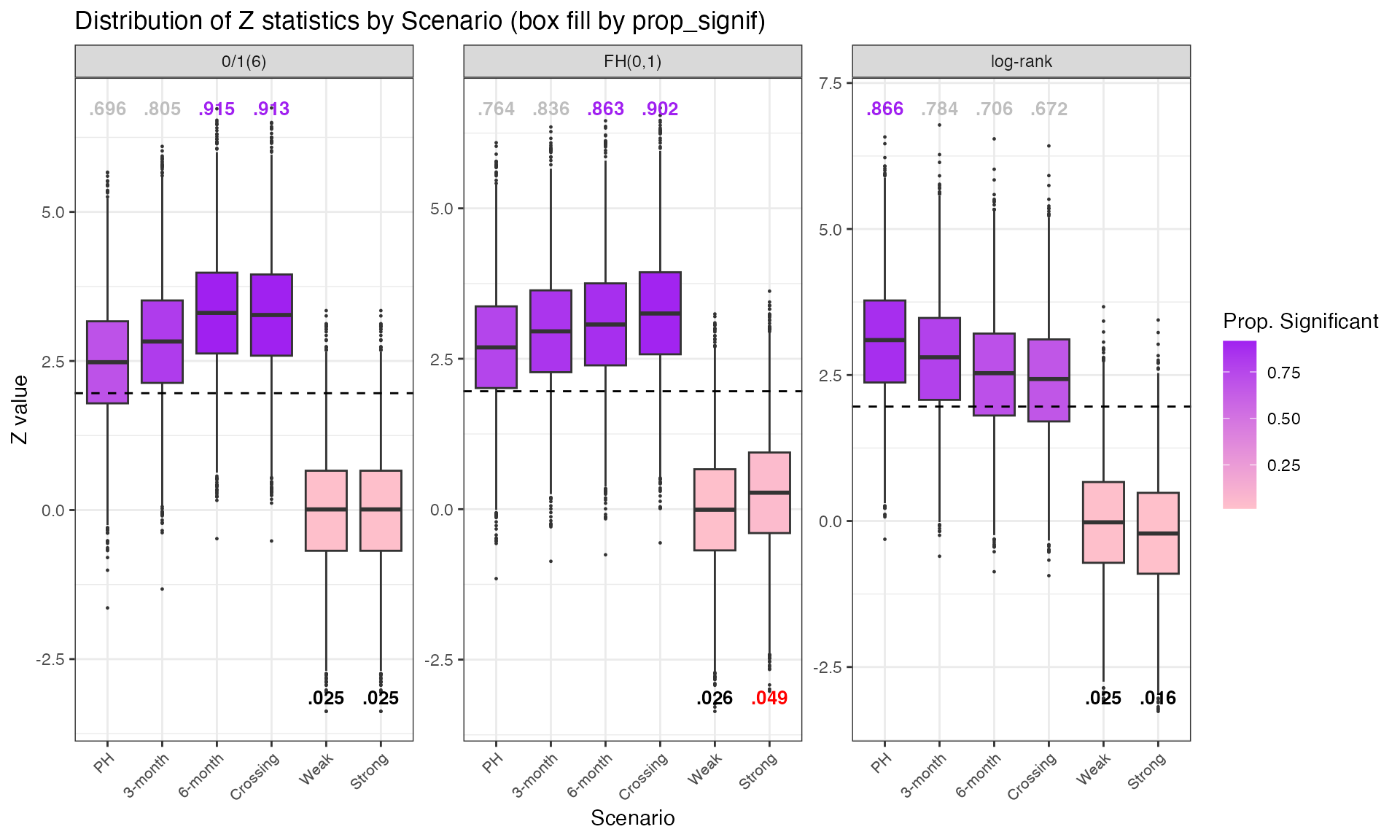
print(p_fill)Wald vs Log-Rank Correspondence
Correspondence between log-rank (weighted log-rank) and Wald (Cox model) tests, evaluated as the proportion of simulations where each test rejects (upper bound for Wald; for log-rank).
| Scenario |
Standard Cox
|
FH(0,1)
|
zero/one(6)
|
|||
|---|---|---|---|---|---|---|
| Wald | logrank | Wald | logrank | Wald | logrank | |
| PH | 0.865 | 0.866 | 0.764 | 0.764 | 0.694 | 0.696 |
| 3m delay | 0.783 | 0.784 | 0.834 | 0.836 | 0.804 | 0.805 |
| 6m delay | 0.705 | 0.706 | 0.861 | 0.863 | 0.915 | 0.915 |
| Crossing | 0.672 | 0.672 | 0.900 | 0.902 | 0.911 | 0.913 |
| Weak null | 0.025 | 0.025 | 0.025 | 0.026 | 0.025 | 0.025 |
| Strong null | 0.016 | 0.016 | 0.047 | 0.049 | 0.025 | 0.025 |
results <- res_out$results_sims
results$Scenario <- factor(results$Scenario, levels = 1:6,
     labels = c("PH", "3m delay", "6m delay", "Crossing",
                "Weak null", "Strong null"))

table_gt <- results %>%
  group_by(Scenario) %>%
  summarise(
    Cox     = mean(fh00_wald < 1.0),
    Logrank = mean(fh00z_mine > qnorm(0.975)),
    Cox01   = mean(fh01_wald < 1.0),
    FH01    = mean(fh01z_mine > qnorm(0.975)),
    Cox601  = mean(t601_wald < 1.0),
    LR601   = mean(t601z > qnorm(0.975))
  ) |>
  gt() |> fmt_number(columns = 2:7, decimals = 3)

table_gt2 <- table_gt %>%
  fmt_number(columns = 2:7, decimals = 3) %>%
  cols_label(
    Cox     = "Wald",
    Logrank = "logrank",
    Cox01   = "Wald ",
    FH01    = "logrank ",
    Cox601  = "Wald  ",
    LR601   = "logrank  "
  ) %>%
  tab_spanner(label = "Standard Cox",  columns = c("Cox", "Logrank")) %>%
  tab_spanner(label = "FH(0,1)",       columns = c("Cox01", "FH01")) %>%
  tab_spanner(label = "zero/one(6)",   columns = c("Cox601", "LR601"))

table_gt3 <- table_gt2 %>%
  tab_style(
    style = cell_fill(color = "#D3D3D3"),
    locations = cells_body(columns = "LR601", rows = Scenario == "6m delay")
  ) %>%
  tab_style(
    style = cell_fill(color = "yellow"),
    locations = cells_body(columns = "Logrank", rows = Scenario == "6m delay")
  )

table_gt3
Cox Hazard Ratio Estimates and SE Estimation
Operating characteristics of Cox hazard-ratio estimates, de-biased estimates, empirical standard errors, and estimated standard errors (asymptotic and de-biased) under standard and zero-one(6) weighting.
| Scenario |
Standard Cox Estimates
|
zero/one(6) Estimators
|
||||||||
|---|---|---|---|---|---|---|---|---|---|---|
| HR | db(HR) | SE | est(SE) | est*(SE) | HR | db(HR) | SE | est(SE) | est*(SE) | |
| PH | 0.762 | 0.755 | 0.091 | 0.090 | 0.085 | 0.762 | 0.755 | 0.112 | 0.112 | 0.110 |
| 3m delay | 0.782 | 0.776 | 0.091 | 0.090 | 0.085 | 0.730 | 0.723 | 0.114 | 0.114 | 0.112 |
| 6m delay | 0.801 | 0.794 | 0.091 | 0.090 | 0.085 | 0.686 | 0.680 | 0.117 | 0.117 | 0.115 |
| Crossing | 0.808 | 0.801 | 0.091 | 0.090 | 0.085 | 0.689 | 0.683 | 0.116 | 0.117 | 0.115 |
| Weak null | 1.005 | 0.997 | 0.087 | 0.086 | 0.082 | 1.006 | 0.997 | 0.109 | 0.110 | 0.110 |
| Strong null | 1.022 | 1.013 | 0.087 | 0.086 | 0.082 | 1.006 | 0.997 | 0.109 | 0.110 | 0.110 |
results <- res_out$results_sims
results$Scenario <- factor(results$Scenario, levels = 1:6,
     labels = c("PH", "3m delay", "6m delay", "Crossing",
                "Weak null", "Strong null"))

table_gt <- results %>%
  group_by(Scenario) %>%
  summarise(
    HR          = mean(exp(fh00_bhat), na.rm = TRUE),
    HR_db       = mean(exp(fh00_bhatdebiased), na.rm = TRUE),
    SE          = sqrt(var(fh00_bhat, na.rm = TRUE)),
    SE_est      = mean(fh00_sigbhat, na.rm = TRUE),
    SE_db       = mean(fh00_sigbhatstar, na.rm = TRUE),
    HR2         = mean(exp(t601_bhat), na.rm = TRUE),
    HR_db2      = mean(exp(t601_bhatdebiased), na.rm = TRUE),
    SE2         = sqrt(var(t601_bhat, na.rm = TRUE)),
    SE_est2     = mean(t601_sigbhat, na.rm = TRUE),
    SE_db2      = mean(t601_sigbhatstar, na.rm = TRUE)
  ) %>%
  gt() %>%
  fmt_number(columns = 2:11, decimals = 3) %>%
  cols_label(
    HR     = "HR",      HR_db   = "db(HR)",
    HR2    = "HR ",     HR_db2  = "db(HR) ",
    SE     = "SE",      SE_est  = "est(SE)",  SE_db  = "est*(SE)",
    SE2    = "SE ",     SE_est2 = "est(SE) ", SE_db2 = "est*(SE) "
  ) %>%
  tab_spanner(label = "Standard Cox Estimates",
              columns = c("HR", "HR_db", "SE", "SE_est", "SE_db")) %>%
  tab_spanner(label = "zero/one(6) Estimators",
              columns = c("HR2", "HR_db2", "SE2", "SE_est2", "SE_db2"))

table_gt2 <- table_gt %>%
  tab_style(
    style = cell_fill(color = "#D3D3D3"),
    locations = cells_body(columns = "HR2", rows = Scenario == "6m delay")
  ) %>%
  tab_style(
    style = cell_fill(color = "yellow"),
    locations = cells_body(columns = "HR", rows = Scenario == "6m delay")
  )

table_gt2
All FH Weighting Variants
Distribution of z-statistics across all implemented weighting variants: FH(0,0), FH(0,0.5), FH(0,1), Magirr-Burman (6 and 12 months), FH-exponential variants (1 and 2), and zero-one(6).
z_main <- c('fh00z_mine', 'fh05z_mine', 'fh01z_mine',
            'mb6z_mine', 'mb12z_mine', 'fhe1z', 'fhe2z', 't601z')

df2 <- res_out$results_sims[, c('Scenario', z_main)]

# Reshape to long format
long_df2 <- tidyr::pivot_longer(df2, cols = -Scenario,
                                 names_to = 'z_stat', values_to = 'z_value')

scenario_labels <- c('PH', '3-month', '6-month', 'Crossing', 'Weak', 'Strong')
long_df2$scenario_name <- factor(long_df2$Scenario,
                                  levels = 1:6, labels = scenario_labels)

ann_df <- long_df2 %>%
  group_by(scenario_name, z_stat) %>%
  summarise(prop_signif = mean(z_value > qnorm(0.975)), .groups = 'drop')

min_z <- long_df2 %>% group_by(z_stat) %>% summarise(min_z = min(z_value))
ann_df_ws <- ann_df %>% filter(scenario_name %in% c('Weak', 'Strong'))
ann_df_ws <- left_join(ann_df_ws, min_z, by = 'z_stat')
ann_df_ws$label <- sub("^0+", "", sub("\\.?0+$", "",
                       sprintf("%.3f", ann_df_ws$prop_signif)))

max_z <- long_df2 %>% group_by(z_stat) %>% summarise(max_z = max(z_value))
ann_df_Nonws <- ann_df %>% filter(!(scenario_name %in% c('Weak', 'Strong')))
ann_df_Nonws <- left_join(ann_df_Nonws, max_z, by = 'z_stat')
ann_df_Nonws$label <- sub("^0+", "", sub("\\.?0+$", "",
                          sprintf("%.3f", ann_df_Nonws$prop_signif)))

n_sim <- res_out$number_sims
pnull_threshold <- round(0.025 + 1.96 * sqrt(0.025 * 0.975 / n_sim), 4)
ann_df_ws$label_color <- ifelse(ann_df_ws$prop_signif > 0.0264, "red", "black")
ann_df_Nonws$label_color <- ifelse(ann_df_Nonws$prop_signif > 0.85,
                                    "purple", "grey")

long_df2_fill <- left_join(long_df2, ann_df, by = c('scenario_name', 'z_stat'))

p_fill_all <- ggplot(long_df2_fill, aes(x = scenario_name, y = z_value,
                                         fill = prop_signif)) +
  geom_boxplot(outlier.size = 0.2) +
  facet_wrap(~z_stat, scales = 'free_y') +
  labs(x = 'Scenario', y = 'Z value',
       title = 'Distribution of Z statistics by Scenario (box fill by prop_signif)',
       fill = 'Prop. Significant') +
  theme_bw() +
  theme(axis.text.x = element_text(angle = 45, hjust = 1, size = 8)) +
  scale_fill_gradient(low = 'yellow', high = 'lightblue') +
  geom_hline(yintercept = qnorm(0.975), linetype = 'dashed',
             color = 'black', linewidth = 0.5) +
  geom_text(data = ann_df_ws, aes(x = scenario_name, y = min_z, label = label,
                                   color = label_color),
            size = 3.5, fontface = 'bold', inherit.aes = FALSE, vjust = -0.5) +
  scale_color_identity() +
  geom_text(data = ann_df_Nonws, aes(x = scenario_name, y = max_z, label = label,
                                      color = label_color),
            size = 3.5, fontface = 'bold', inherit.aes = FALSE, vjust = 0.5)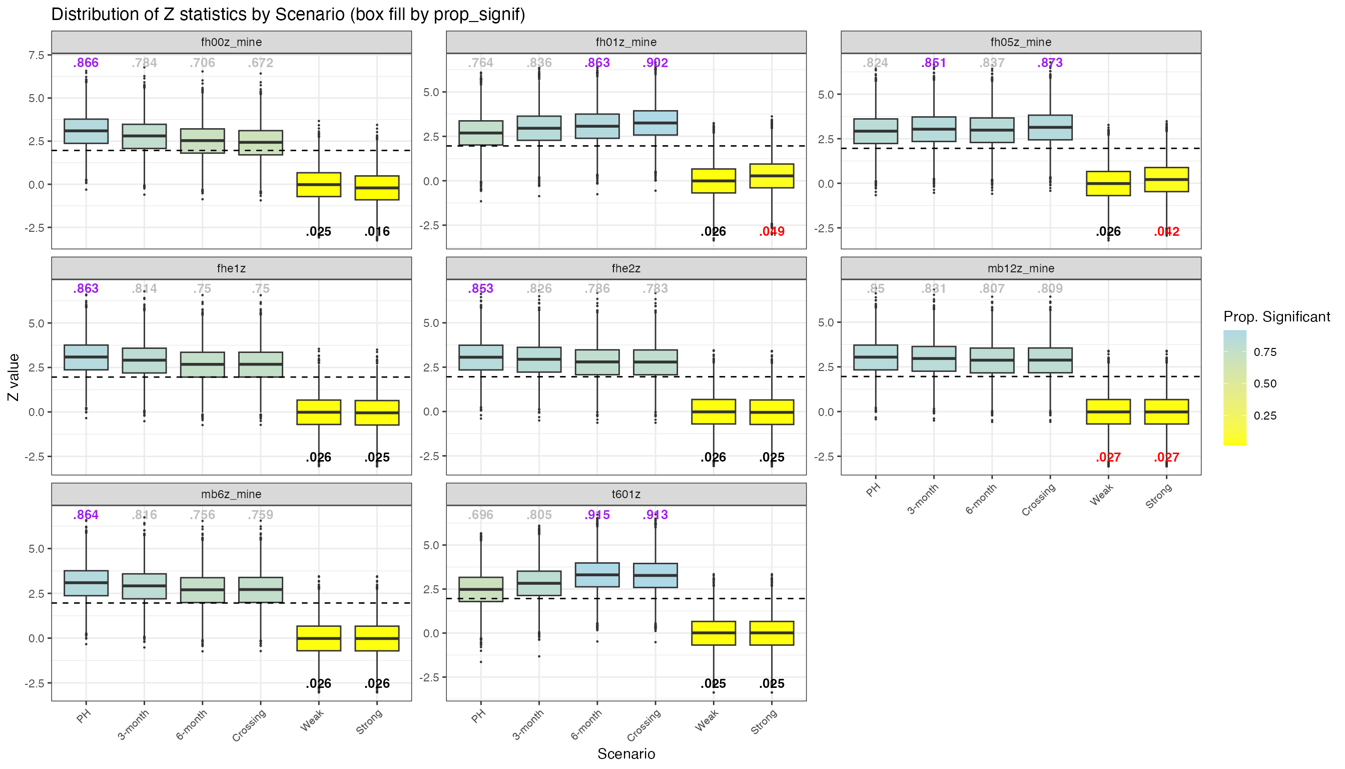
print(p_fill_all)Checking Alignment with simtrial
To validate weightedsurv implementations, we compare
z-statistics computed by weightedsurv (suffix
_mine) against those produced by simtrial for
the same simulated datasets. Paired facets (e.g., logrankz
vs fh00z_mine, mb6z vs mb6z_mine)
should show near-identical distributions.
# Full comparison of all z-statistics: simtrial vs weightedsurv
z_cols <- grep('z', colnames(res_out$results_sims), value = TRUE)
z_cols_nondebiased <- z_cols[!grepl('debiased', z_cols)]
df2 <- res_out$results_sims[, c('Scenario', z_cols_nondebiased)]

long_df2 <- tidyr::pivot_longer(df2, cols = -Scenario,
                                 names_to = 'z_stat', values_to = 'z_value')

# Custom order: group simtrial and weightedsurv variants together
z_main <- c('logrankz', 'fh00z_mine', 'fh05z', 'fh05z_mine', 'fh01z', 'fh01z_mine',
            'mb6z', 'mb6z_mine', 'mb12z', 'mb12z_mine', 'fhe1z', 'fhe2z', 't601z')

z_order2 <- z_main[z_main %in% z_cols_nondebiased]
z_order2 <- c(z_order2, setdiff(z_cols_nondebiased, z_order2))
long_df2$z_stat <- factor(long_df2$z_stat, levels = z_order2)

scenario_labels <- c('PH', '3-month', '6-month', 'Crossing', 'Weak', 'Strong')
long_df2$scenario_name <- factor(long_df2$Scenario,
                                  levels = 1:6, labels = scenario_labels)

ann_df <- long_df2 %>%
  group_by(scenario_name, z_stat) %>%
  summarise(prop_signif = mean(z_value > qnorm(0.975)), .groups = 'drop')

min_z <- long_df2 %>% group_by(z_stat) %>% summarise(min_z = min(z_value))
ann_df_ws <- ann_df %>% filter(scenario_name %in% c('Weak', 'Strong'))
ann_df_ws <- left_join(ann_df_ws, min_z, by = 'z_stat')
ann_df_ws$label <- sub("^0+", "", sub("\\.?0+$", "",
                       sprintf("%.3f", ann_df_ws$prop_signif)))

n_sim <- res_out$number_sims
pnull_threshold <- round(0.025 + 1.96 * sqrt(0.025 * 0.975 / n_sim), 4)
ann_df_ws$label_color <- ifelse(ann_df_ws$prop_signif > 0.0264, "red", "black")

long_df2_fill <- left_join(long_df2, ann_df, by = c('scenario_name', 'z_stat'))

p_fill_compare <- ggplot(long_df2_fill, aes(x = scenario_name, y = z_value,
                                              fill = prop_signif)) +
  geom_boxplot(outlier.size = 0.2) +
  facet_wrap(~z_stat, scales = 'free_y') +
  labs(x = 'Scenario', y = 'Z value',
       title = 'Distribution of Z statistics by Scenario (box fill by prop_signif)',
       fill = 'Prop. Significant') +
  theme_bw() +
  theme(axis.text.x = element_text(angle = 45, hjust = 1, size = 8)) +
  scale_fill_gradient(low = 'yellow', high = 'lightblue') +
  geom_hline(yintercept = qnorm(0.975), linetype = 'dashed',
             color = 'black', linewidth = 0.5) +
  geom_text(data = ann_df_ws, aes(x = scenario_name, y = min_z, label = label,
                                   color = label_color),
            size = 3.5, fontface = 'bold', inherit.aes = FALSE, vjust = -0.5) +
  scale_color_identity()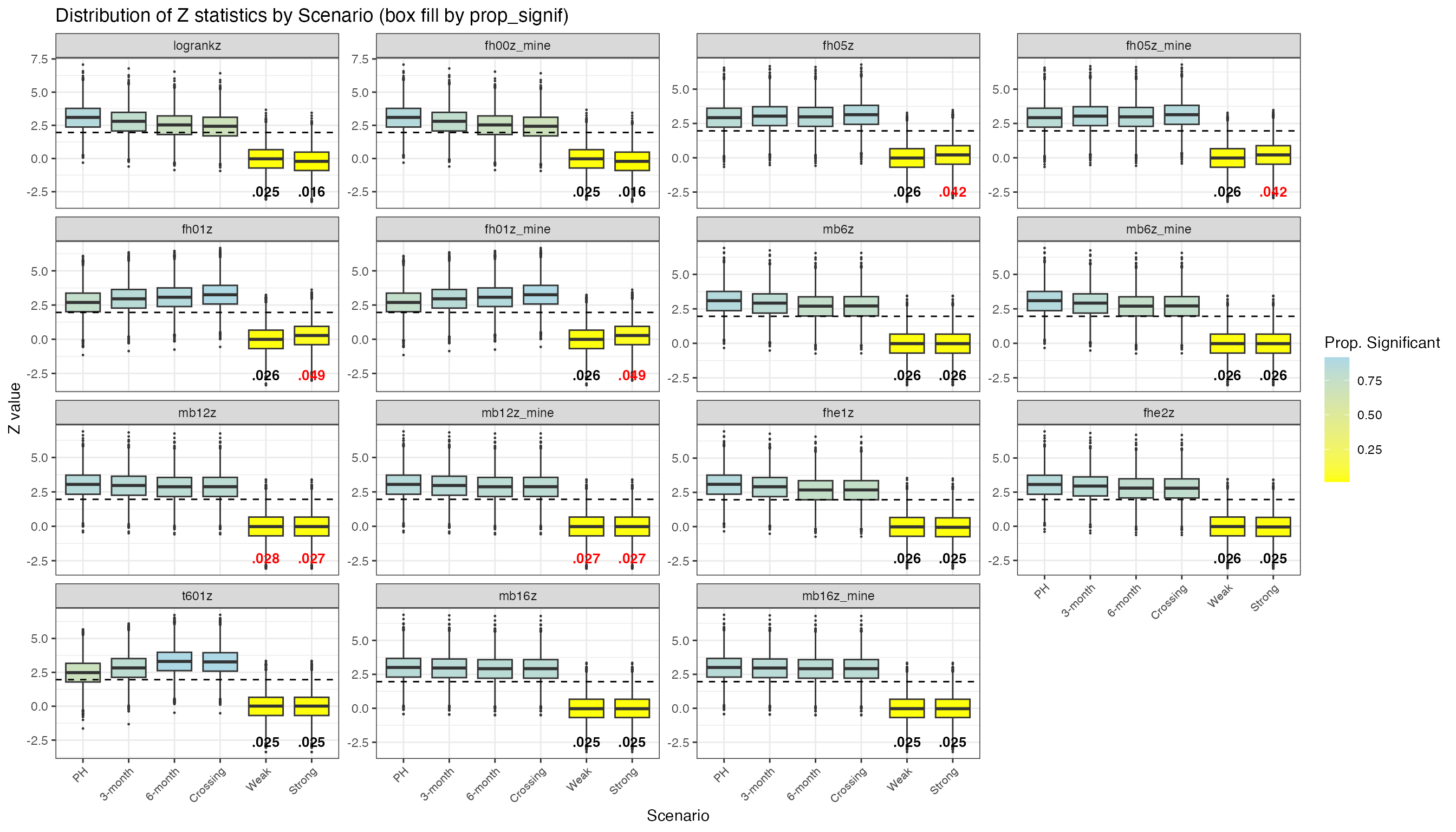
print(p_fill_compare)