Exploratory Subgroup Identification with ForestSearch

Introduction

This vignette demonstrates the ForestSearch methodology for exploratory subgroup identification in survival analysis, as described in León et al. (2024) Statistics in Medicine.

Motivation

In clinical trials, particularly oncology, subgroup analyses are essential for:

Evaluating treatment effect consistency across patient populations
Identifying subgroups where treatment may be detrimental (harm)
Characterizing subgroups with enhanced benefit
Informing regulatory decisions and clinical practice

While prespecified subgroups provide stronger evidence, important subgroups based on patient characteristics may not be anticipated. ForestSearch provides a principled approach to exploratory subgroup identification with proper statistical inference.

Methodology Overview

ForestSearch identifies subgroups through:

Candidate factor selection: Using LASSO and/or Generalized Random Forests (GRF)
Exhaustive subgroup search: Evaluating all combinations up to maxk factors
Consistency-based selection: Applying splitting consistency criteria
Bootstrap bias correction: Adjusting for selection-induced optimism
Cross-validation: Assessing algorithm stability

The key innovation is the splitting consistency criterion: a subgroup is considered “consistent with harm” if, when randomly split 50/50 many times, both halves consistently show hazard ratios ≥ 1.0 (for example if 1.0 represents a meaningful “harm threshold”).

Setup

Load Required Packages

library(forestsearch)
library(survival)
library(data.table)
library(ggplot2)
library(gt)
library(grf)
library(policytree)
library(doFuture)

# Optional packages for enhanced output
library(patchwork)
library(weightedsurv)

# Set ggplot theme
theme_set(theme_minimal(base_size = 12))

Data: German Breast Cancer Study Group Trial

Study Background

The GBSG trial evaluated hormonal treatment (tamoxifen) versus chemotherapy in node-positive breast cancer patients. Key characteristics:

Sample size: N = 686
Outcome: Recurrence-free survival time
Censoring rate: ~56%
Treatment: Hormonal therapy (tamoxifen) vs. chemotherapy

Data Preparation

# Load GBSG data (included in forestsearch package)
df.analysis <- gbsg

# Prepare analysis variables
df.analysis <- within(df.analysis, {
  id <- seq_len(nrow(df.analysis))
  time_months <- rfstime / 30.4375
  grade3 <- ifelse(grade == "3", 1, 0)
  treat <- hormon
})

# Define variable roles
confounders.name <- c("age", "meno", "size", "grade3", "nodes", "pgr", "er")
outcome.name <- "time_months"
event.name <- "status"
id.name <- "id"
treat.name <- "hormon"

# Display data structure
cat("Sample size:", nrow(df.analysis), "\n")

## Sample size: 686

cat("Events:", sum(df.analysis[[event.name]]), 
    sprintf("(%.1f%%)\n", 100 * mean(df.analysis[[event.name]])))

## Events: 299 (43.6%)

cat("Baseline factors:", paste(confounders.name, collapse = ", "), "\n")

## Baseline factors: age, meno, size, grade3, nodes, pgr, er

Baseline Characteristics

create_summary_table(
  data = df.analysis,
  treat_var = treat.name,
  table_title = "GBSG Baseline Characteristics by Treatment Arm",
  vars_continuous = c("age", "nodes", "size", "er", "pgr"),
  vars_categorical = c("grade", "meno"),
  font_size = 12
)

Characteristic		Control (n=440)	Treatment (n=246)	P-value¹	SMD²
GBSG Baseline Characteristics by Treatment Arm
age	Mean (SD)	51.1 (10.0)	56.6 (9.4)	<0.001	0.57
nodes	Mean (SD)	4.9 (5.6)	5.1 (5.3)	0.665	0.03
size	Mean (SD)	29.6 (14.4)	28.8 (14.1)	0.470	0.06
er	Mean (SD)	79.7 (124.2)	125.8 (191.1)	<0.001	0.30
pgr	Mean (SD)	102.0 (170.0)	124.3 (249.7)	0.213	0.11
grade				0.273	0.06
	1	48 (10.9%)	33 (13.4%)
	2	281 (63.9%)	163 (66.3%)
	3	111 (25.2%)	50 (20.3%)
meno				<0.001	0.27
	0	231 (52.5%)	59 (24.0%)
	1	209 (47.5%)	187 (76.0%)
¹ P-values: t-test for continuous, chi-square/Fisher's exact for categorical/binary variables
² SMD = Standardized mean difference (Cohen's d for continuous, Cramer's V for categorical)

Kaplan-Meier Analysis (ITT Population)

# Prepare counting process data for KM plot
dfcount <- df_counting(
  df = df.analysis,
  by.risk = 6,
  tte.name = outcome.name,
  event.name = event.name,
  treat.name = treat.name
)

# Plot with confidence intervals and log-rank test
plot_weighted_km(
  dfcount,
  conf.int = TRUE,
  show.logrank = TRUE,
  ymax = 1.05,
  xmed.fraction = 0.775,
  ymed.offset = 0.125
)

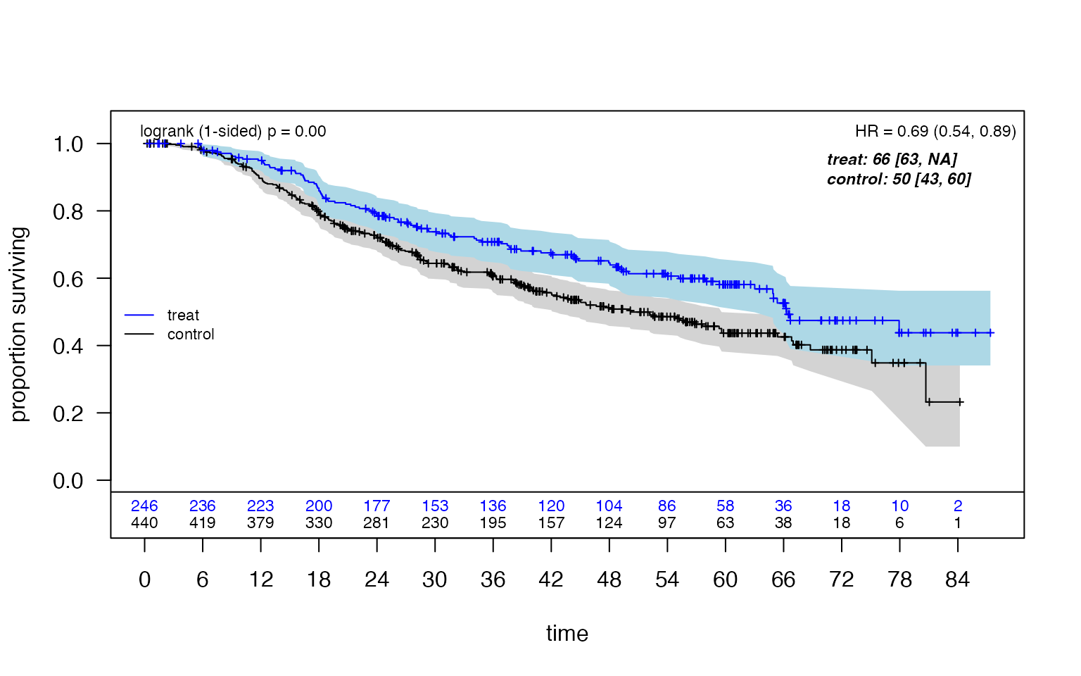
The ITT Cox hazard ratio estimate is approximately 0.69 (95% CI: 0.54, 0.89), suggesting an overall benefit for hormonal therapy.

Preliminary Analysis: Generalized Random Forests

Before running ForestSearch, we can use GRF to explore potential treatment effect heterogeneity and identify candidate factors.

t0 <- proc.time()

grf_est <- grf.subg.harm.survival(
  data = df.analysis,
  confounders.name = confounders.name,
  outcome.name = outcome.name,
  event.name = event.name,
  id.name = id.name,
  treat.name = treat.name,
  maxdepth = 2,
  n.min = 60,
  dmin.grf = 12,
  frac.tau = 0.6,
  details = TRUE,
  return_selected_cuts_only = FALSE
)

## tau, maxdepth = 46.75811 2 
##    leaf.node control.mean control.size control.se depth
## 1          2         6.49        82.00       3.34     1
## 2          3        -4.10       604.00       1.06     1
## 11         4        -7.90       112.00       2.81     2
## 21         5         3.86       177.00       1.87     2
## 4          7        -5.89       356.00       1.33     2
## 
## Selected subgroup:
##   leaf.node control.mean control.size control.se depth
## 1         2         6.49        82.00       3.34     1
## 
## GRF subgroup found
## Terminating node at max.diff (sg.harm.id):
## [1] "er <= 0"
## 
## All splits (from all trees):
## [1] "er <= 0"   "age <= 50" "age <= 43"

timings$grf <- (proc.time() - t0)["elapsed"]

# Display policy trees
# leaf1 = recommend control, leaf2 = recommend treatment
par(mfrow = c(1, 2))
plot(grf_est$tree1, leaf.labels = c("Control", "Treat"), main = "Depth 1")

plot(grf_est$tree2, leaf.labels = c("Control", "Treat"), main = "Depth 2")

par(mfrow = c(1, 1))

GRF identifies estrogen receptor status (ER) as a key factor, with ER ≤ 0 suggesting potential harm from hormonal therapy.

ForestSearch Analysis

Parallel Processing Configuration

ForestSearch supports parallel processing for computationally intensive operations (bootstrap, cross-validation).

# Detect available cores (limited to 2 cores for CRAN checks)
n_cores <- 2
n_cores_total <- parallel::detectCores()
cat("Using", n_cores, "of", n_cores_total, "total cores for parallel processing")

## Using 2 of 14 total cores for parallel processing

Running ForestSearch

ForestSearch performs an exhaustive search over candidate subgroup combinations with up to maxk factors. Key parameters:

Parameter	Value	Description
`hr.threshold`	1.25	Minimum HR for consistency evaluation
`hr.consistency`	1.0	Minimum consistency rate for candidates
`pconsistency.threshold`	0.90	Required consistency for selection
`maxk`	2	Maximum factors in subgroup definition
`n.min`	60	Minimum subgroup sample size
`d0.min`, `d1.min`	12	Minimum events per treatment arm

t0 <- proc.time()

fs <- forestsearch(
  df.analysis,
  confounders.name = confounders.name,
  outcome.name = outcome.name,
  treat.name = treat.name,
  event.name = event.name,
  id.name = id.name,
  # Threshold parameters (per León et al. 2024)
  hr.threshold = 1.25,
  hr.consistency = 1.0,
  pconsistency.threshold = 0.80,
  stop_threshold = 0.80,
  # Search configuration
  sg_focus = "hr",
  max_subgroups_search = 3,
  use_twostage = TRUE,
  # Factor selection
  use_grf = TRUE, 
  return_selected_cuts_only = TRUE,
  use_lasso = TRUE,
  cut_type = "default",
  # Subgroup constraints
  maxk = 2,
  n.min = 60,
  d0.min = 12,
  d1.min = 12,
  # Consistency evaluation
  fs.splits = 100,
  # Parallel processing
  parallel_args = list(
    plan = "multisession",
    workers = n_cores,
    show_message = TRUE
  ),
  # Output options
  showten_subgroups = TRUE,
  details = TRUE,
  plot.sg = TRUE
)

## 
## === Two-Stage Consistency Evaluation Enabled ===
## Stage 1 screening splits: 30 
## Maximum total splits: 100 
## Batch size: 20 
## ================================================
## 
## GRF stage for cut selection with dmin, tau = 12 0.6 
##   return_selected_cuts_only = TRUE: using cuts from selected tree only
## tau, maxdepth = 46.75811 2 
##    leaf.node control.mean control.size control.se depth
## 1          2         6.49        82.00       3.34     1
## 2          3        -4.10       604.00       1.06     1
## 11         4        -7.90       112.00       2.81     2
## 21         5         3.86       177.00       1.87     2
## 4          7        -5.89       356.00       1.33     2
## 
## Selected subgroup:
##   leaf.node control.mean control.size control.se depth
## 1         2         6.49        82.00       3.34     1
## 
## GRF subgroup found
## Terminating node at max.diff (sg.harm.id):
## [1] "er <= 0"
## 
## Cuts from selected tree (depth = 1 ):
## [1] "er <= 0"
## GRF cuts identified: 1 
##   Cuts: er <= 0 
##   Selected tree depth: 1 
## # of continuous/categorical characteristics 5 2 
## Continuous characteristics: age size nodes pgr er 
## Categorical characteristics: meno grade3 
## ## Prior to lasso: age size nodes pgr er 
## #### Lasso selection results 
## 7 x 1 sparse Matrix of class "dgCMatrix"
##                  s0
## age     .          
## meno    .          
## size    0.005433435
## grade3  0.178139021
## nodes   0.049670523
## pgr    -0.001812895
## er      .          
## Cox-LASSO selected: size grade3 nodes pgr 
## Cox-LASSO not selected: age meno er 
## ### End Lasso selection 
## ## After lasso: size nodes pgr 
## Default cuts included from Lasso: size <= mean(size) size <= median(size) size <= qlow(size) size <= qhigh(size) nodes <= mean(nodes) nodes <= median(nodes) nodes <= qlow(nodes) nodes <= qhigh(nodes) pgr <= mean(pgr) pgr <= median(pgr) pgr <= qlow(pgr) pgr <= qhigh(pgr) 
## Categorical after Lasso: grade3 
## Factors per GRF: er <= 0 
## Initial GRF cuts included er <= 0 
## Factors included per GRF (not in lasso) er <= 0 
## 
## ===== CONSOLIDATED CUT EVALUATION (IMPROVED) =====
## Evaluating 14 cut expressions once and caching...
## Cut evaluation summary:
##   Total cuts:  14 
##   Valid cuts:  14 
##   Errors:  0 
## ✓ All 14 factors validated as 0/1
## ===== END CONSOLIDATED CUT EVALUATION =====
## 
## # of candidate subgroup factors= 14 
##  [1] "er <= 0"      "size <= 29.3" "size <= 25"   "size <= 20"   "size <= 35"  
##  [6] "nodes <= 5"   "nodes <= 3"   "nodes <= 1"   "nodes <= 7"   "pgr <= 110"  
## [11] "pgr <= 32.5"  "pgr <= 7"     "pgr <= 131.8" "grade3"      
## Number of possible configurations (<= maxk): maxk = 2 , # combinations = 406 
## Events criteria: control >= 12 , treatment >= 12 
## Sample size criteria: n >= 60 
## Subgroup search completed in 0.01 minutes
## 
## --- Filtering Summary ---
##   Combinations evaluated: 406 
##   Passed variance check: 374 
##   Passed prevalence (>= 0.025 ): 374 
##   Passed redundancy check: 354 
##   Passed event counts (d0>= 12 , d1>= 12 ): 250 
##   Passed sample size (n>= 60 ): 247 
##   Cox model fit successfully: 247 
##   Passed HR threshold (>= 1.25 ): 7 
## -------------------------
## 
## Found 7 subgroup candidate(s)
## # of candidate subgroups (meeting all criteria) = 7 
## Random seed set to: 8316951 
## Two-stage parameters:
##   n.splits.screen: 30 
##   screen.threshold: 0.617 
##   batch.size: 20 
##   conf.level: 0.95 
## # of unique initial candidates: 7 
## # Restricting to top stop_Kgroups = 3 
## # of candidates to evaluate: 3 
## # Early stop threshold: 0.8 
## 
## ================================================================================ 
## TOP 3 CANDIDATE SUBGROUPS FOR CONSISTENCY EVALUATION
## Sorted by: hr 
## ================================================================================ 
## 
## Rank   HR        N       Events  K    Subgroup Definition
## -------------------------------------------------------------------------------- 
## 1      2.537     61      34      2    {er <= 0} & {size <= 35}
## 2      2.222     75      41      2    {er <= 0} & {pgr <= 32.5}
## 3      2.054     61      35      2    {er <= 0} & !{size <= 20}
## --------------------------------------------------------------------------------

## Parallel config: workers = 2 , batch_size = 1 
## Batch 1 / 3 : candidates 1 - 1 
## 
## ==================================================
## EARLY STOP TRIGGERED (batch 1 )
##   Candidate: 1 of 3 
##   Pcons: 0.97 >= 0.8 
## ==================================================
## 
## Evaluated 1 of 3 candidates (early stop) 
## 1 subgroups passed consistency threshold

## *** Subgroup found: {er <= 0} {size <= 35} 
## % consistency criteria met= 0.97 
## SG focus = hr 
## Seconds and minutes forestsearch overall = 1.962 0.0327 
## Consistency algorithm used: twostage

plan("sequential")
timings$forestsearch <- (proc.time() - t0)["elapsed"]

cat("\nForestSearch completed in", 
    round(timings$forestsearch, 1), "seconds\n")

## 
## ForestSearch completed in 2 seconds

ForestSearch Results

Identified Subgroups

# Generate results tables
res_tabs <- sg_tables(fs, ndecimals = 3, which_df = "est")

# Display top subgroups meeting criteria
res_tabs$sg10_out

Factor 1	Factor 2	N	Events	E₁	HR	P_cons
Identified Subgroups
Two-factor subgroups (maxk=2)
{er <= 0}	{size <= 35}	61	34	15	2.537	0.970
Search Configuration: Single-factor candidates (L) = 28; Maximum combinations evaluated = 406; Search depth (maxk) = 2
Search Results: Candidate subgroups found = 7; Maximum HR estimate = 2.54
Note: E₁ = events in treatment arm; P_cons = consistency proportion

Treatment Effect Estimates

# ITT and subgroup estimates
res_tabs$tab_estimates

Subgroup	n	n1	events	m1	m0	RMST	HR (95% CI)
Treatment Effect Estimates
Training data estimates
ITT	686 (100.0%)	246 (35.9%)	299 (43.6%)	66.3	50.2	7.8	0.69 (0.54, 0.89)
Questionable¹	61 (8.9%)	23 (37.7%)	34 (55.7%)	18.5	48	-19	2.54 (1.25, 5.17)
Recommend	625 (91.1%)	223 (35.7%)	265 (42.4%)	66.7	52.2	9.6	0.61 (0.47, 0.79)
¹ Identified subgroup : {er <= 0} & {size <= 35}

Identified Subgroup Definition

cat("Identified subgroup (H):", paste(fs$sg.harm, collapse = " & "), "\n")

## Identified subgroup (H): {er <= 0} & {size <= 35}

cat("Subgroup size:", sum(fs$df.est$treat.recommend == 0), 
    sprintf("(%.1f%% of ITT)\n", 
            100 * mean(fs$df.est$treat.recommend == 0)))

## Subgroup size: 61 (8.9% of ITT)

ForestSearch identifies Estrogen ≤ 0 (ER-negative) as the subgroup with potential harm. This is biologically plausible: tamoxifen is a selective estrogen receptor modulator with limited efficacy in ER-negative tumors.

Bootstrap Bias Correction

Rationale

Cox model estimates from identified subgroups are upwardly biased due to the selection process (subgroups are selected because they show extreme effects). Bootstrap bias correction addresses this by:

Resampling with replacement
Re-running the entire ForestSearch algorithm
Computing bias terms from bootstrap vs. observed estimates
Applying infinitesimal jackknife variance estimation

Running Bootstrap Analysis

# Number of bootstrap iterations
# Use 500-2000 for production; reduced here for vignette
NB <- 2

t0 <- proc.time()

fs_bc <- forestsearch_bootstrap_dofuture(
  fs.est = fs,
  nb_boots = NB,
  show_three = FALSE,
  details = FALSE,
  parallel_args = list(
    plan = "multisession",
    workers = n_cores,
    show_message = TRUE
  )
)

plan("sequential")
timings$bootstrap <- (proc.time() - t0)["elapsed"]

cat("\nBootstrap completed in", 
    round(timings$bootstrap / 60, 1), "minutes\n")

## 
## Bootstrap completed in 0.1 minutes

Bootstrap Summary and Diagnostics

# Comprehensive summary with diagnostics
summaries <- summarize_bootstrap_results(
  sgharm = fs$sg.harm,
  boot_results = fs_bc,
  create_plots = TRUE,
  est.scale = "hr"
)

## 
## ===============================================================
##            BOOTSTRAP ANALYSIS SUMMARY                          
## ===============================================================
## 
## IDENTIFIED SUBGROUP:
## -------------------------------------------------------------
##   H: {er <= 0} & {size <= 35}
## 
## BOOTSTRAP SUCCESS METRICS:
## -------------------------------------------------------------
##   Total iterations:              2
##   Successful subgroup ID:        2 (100.0%)
##   Failed to find subgroup:       0 (0.0%)
## 
## TIMING ANALYSIS:
## -------------------------------------------------------------
## Overall:
##   Total bootstrap time:          0.04 minutes (0.00 hours)
##   Average per iteration:         0.02 min (1.1 sec)
##   Projected for 1000 boots:      18.77 min (0.31 hrs)

# Display bias-corrected estimates table
summaries$table

Subgroup	Sample Size			Survival			Treatment Effect
Treatment Effect by Subgroup
Bootstrap bias-corrected estimates (2 iterations)
Subgroup	N	N_T	Events	Med_T	Med_C	RMST_d	HR (95% CI)^†¹	HR^‡ (95% CI)²
Qstnbl³	61 (8.9%)	23 (37.7%)	34 (55.7%)	18.5	48	-19	2.54 (1.25, 5.17)	2.13 (0.15,29.84)
Recmnd	625 (91.1%)	223 (35.7%)	265 (42.4%)	66.7	52.2	9.6	0.61 (0.47, 0.79)	0.57 (0.08,3.95)
¹ Unadjusted HR: Standard Cox regression hazard ratio with robust standard errors
² Bias-corrected HR: Bootstrap-adjusted estimate using infinitesimal jackknife method (2 iterations). Corrects for optimism in subgroup selection.
³ Identified subgroup: {er <= 0} & {size <= 35}
Note: Med = Median survival time (months). RMST_d = Restricted mean survival time difference. Subgroup identified in 100.0% of bootstrap samples.

Kaplan-Meier by Identified Subgroups

 km_result <- plot_sg_weighted_km(
   fs.est = fs,
   outcome.name = "time_months",
   event.name = "status",
   treat.name = "hormon",
   show.logrank = FALSE,
   conf.int = TRUE,
   by.risk = 12,
   show.cox = FALSE, show.cox.bc = TRUE,
   fs_bc = fs_bc,
   hr_bc_position = "topright"
 )

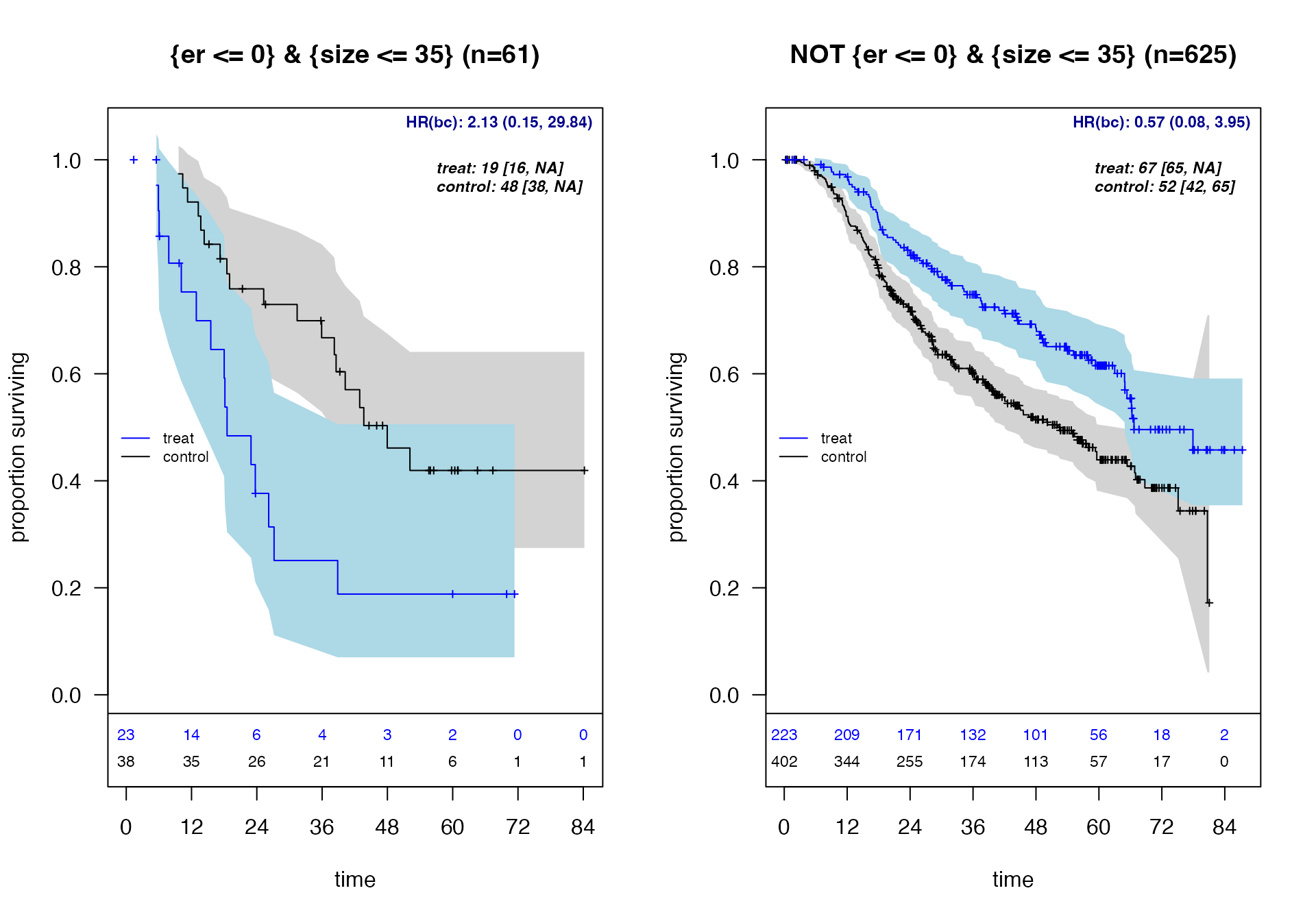
Kaplan-Meier survival curves by identified subgroup

Note: Identified subgroup: {er <= 0} & {size <= 35}. HR(bc) = bootstrap bias-corrected hazard ratio. Medians [95% CI] for arms are un-adjusted.

Event Count Summary

Low event counts can lead to unstable HR estimates. This summary helps identify potential issues:

# note that default required minimum events is 12 for subgroup candidate
# Here we evaluate frequency of subgroup candidates in bootstrap samples less than 15
event_summary <- summarize_bootstrap_events(fs_bc, threshold = 15)

## 
## === Bootstrap Event Count Summary ===
## Total bootstrap iterations: 2
## Event threshold: <15 events
## 
## ORIGINAL Subgroup H on BOOTSTRAP samples:
##   Control arm <15 events: 0 (0.0%)
##   Treatment arm <15 events: 0 (0.0%)
##   Either arm <15 events: 0 (0.0%)
## 
## ORIGINAL Subgroup Hc on BOOTSTRAP samples:
##   Control arm <15 events: 0 (0.0%)
##   Treatment arm <15 events: 0 (0.0%)
##   Either arm <15 events: 0 (0.0%)
## 
## NEW Subgroups found: 2 (100.0%)
## 
## NEW Subgroup H* on ORIGINAL data:
##   Control arm <15 events: 1 (50.0% of successful)
##   Treatment arm <15 events: 1 (50.0% of successful)
##   Either arm <15 events: 1 (50.0% of successful)
## 
## NEW Subgroup Hc* on ORIGINAL data:
##   Control arm <15 events: 0 (0.0% of successful)
##   Treatment arm <15 events: 0 (0.0% of successful)
##   Either arm <15 events: 0 (0.0% of successful)

Bootstrap Diagnostics

# Quality metrics
summaries$diagnostics_table_gt

Category	Metric	Value
Bootstrap Diagnostics Summary
Analysis of 2 bootstrap iterations
Success Rate	Total iterations	2
	Successful	2 (100.0%)
	Failed	0 (0.0%)
	Success rating	Excellent
Subgroup H (Questionable)	Observed HR	2.537
	Bias-corrected HR	2.131
	Bootstrap CV (%)	60.2%
	N estimates	2
Subgroup Hc (Recommend)	Observed HR	0.608
	Bias-corrected HR	0.570
	Bootstrap CV (%)	59.4%
	N estimates	2

Subgroup Agreement

How consistently does bootstrap identify the same subgroup?

# Agreement with original analysis
if (!is.null(summaries$subgroup_summary$original_agreement)) {
  summaries$subgroup_summary$original_agreement
}

##                             Metric                    Value
##                             <char>                   <char>
## 1:      Total bootstrap iterations                        2
## 2:           Successful iterations                        2
## 3: Failed iterations (no subgroup)                        0
## 4:                                                         
## 5:    Original subgroup definition {er <= 0} & {size <= 35}
## 6:       Exact match with original                 0 (0.0%)
## 7:         Different from original               2 (100.0%)
## 8:   Partial match (shared factor)                 0 (0.0%)

# Factor presence across bootstrap iterations
if (!is.null(summaries$subgroup_summary$factor_presence)) {
  summaries$subgroup_summary$factor_presence
}

##   Rank Factor Count Percent
## 1    1    age     1      50
## 2    2 grade3     1      50
## 3    3    pgr     1      50
## 4    4   size     1      50

Bootstrap Distributions

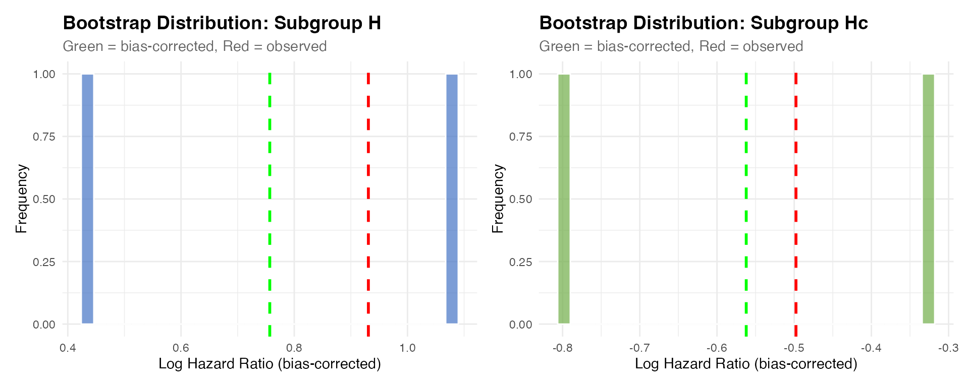
if (!is.null(summaries$plots)) {
  summaries$plots$H_distribution + summaries$plots$Hc_distribution
}

Cross-Validation

Cross-validation assesses the stability of the ForestSearch algorithm. Two approaches are available:

K-Fold Cross-Validation

# 10-fold CV with multiple iterations
# Use Ksims >= 50 for production
Ksims <- 1

t0 <- proc.time()

fs_kfold <- forestsearch_tenfold(
  fs.est = fs,
  sims = Ksims,
  Kfolds = 2,
  details = FALSE,
  parallel_args = list(
    plan = "multisession",
    workers = n_cores,
    show_message = FALSE
  )
)

plan("sequential")
timings$kfold <- (proc.time() - t0)["elapsed"]
metrics_tables <- cv_metrics_tables(fs_kfold)
metrics_tables

Metric	Description	Value (%)
Cross-Validation Metrics
Subgroup: Identified Subgroup
Agreement
Sensitivity (H)	Agreement rate for subgroup H	11.5
Sensitivity (Hc)	Agreement rate for complement Hc	89.8
PPV (H)	Positive predictive value for H	9.9
PPV (Hc)	Positive predictive value for Hc	91.2
Subgroup Finding
Any Found	Any subgroup identified	50.0
Exact Match	Exact match on all factors	0.0
At Least 1	At least one factor matches	50.0
Cov1 Any	First covariate found (any cut)	0.0
Cov2 Any	Second covariate found (any cut)	50.0
Cov1 & Cov2	Both covariates found	0.0
Cov1 Exact	First covariate exact match	0.0
Cov2 Exact	Second covariate exact match	50.0
Based on 1 simulation(s) with 2-fold CV. Values are proportions shown as percentages.

Out-of-Bag (N-Fold) Cross-Validation

N-fold CV (leave-one-out):

t0 <- proc.time()

fs_OOB <- forestsearch_Kfold(
  fs.est = fs,
  details = FALSE,
  Kfolds = round(nrow(df.analysis)/100,0),  # N-fold = leave-one-out
  parallel_args = list(
    plan = "multisession",
    workers = n_cores,
    show_message = TRUE
  )
)

plan("sequential")
timings$oob <- (proc.time() - t0)["elapsed"]

# Summarize OOB results
cv_out <- forestsearch_KfoldOut(
  res = fs_OOB,
  details = FALSE,
  outall = TRUE
)

tables <- cv_summary_tables(cv_out)

tables$combined_table

tables$metrics_table

Results Visualization

Forest Plot

The forest plot summarizes treatment effects across the ITT population, reference subgroups, and identified subgroups with cross-validation metrics.

# Define reference subgroups for comparison
subgroups <- list(
  age_gt65 = list(
    subset_expr = "age > 65",
    name = "Age > 65",
    type = "reference"
  ),
  age_le65 = list(
    subset_expr = "age <= 65",
    name = "Age ≤ 65",
    type = "reference"
  ),
  pgr_positive = list(
    subset_expr = "pgr > 0",
    name = "PgR > 0",
    type = "reference"
  ),
  pgr_negative = list(
    subset_expr = "pgr <= 0",
    name = "PgR ≤ 0",
    type = "reference"
  )
)


my_theme <- create_forest_theme(base_size = 24, 
footnote_fontsize = 17, cv_fontsize = 22)


# Create forest plot
# Include fs_kfold and fs_OOB if available for CV metrics
result <- plot_subgroup_results_forestplot(
  fs_results = list(
    fs.est = fs,
    fs_bc = fs_bc,
    fs_OOB = NULL,
    fs_kfold = fs_kfold
  ),
  df_analysis = df.analysis,
  subgroup_list = subgroups,
  outcome.name = outcome.name,
  event.name = event.name,
  treat.name = treat.name,
  E.name = "Hormonal",
  C.name = "Chemo",
  ci_column_spaces = 25,
  xlog = TRUE,
  theme = my_theme
)


# Option 2: Custom sizing
render_forestplot(result)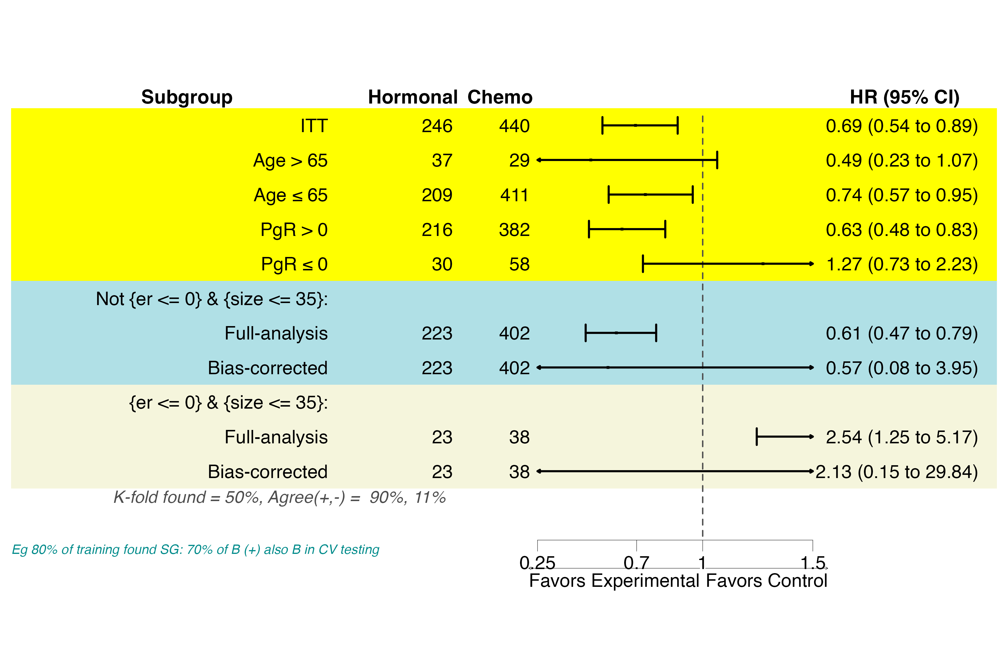

Subgroup forest plot including identified subgroups

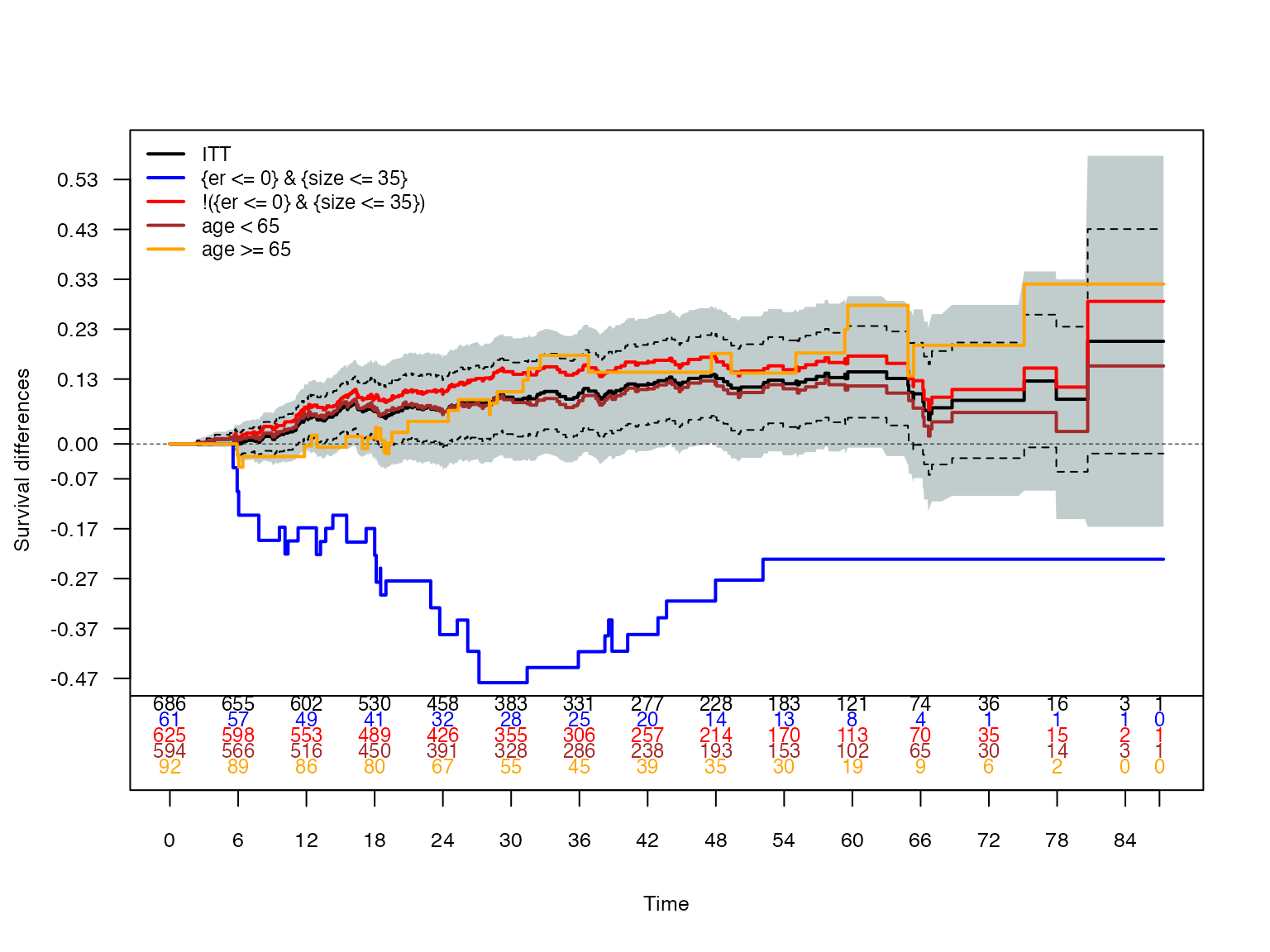
KM Difference plots: ITT and subgroups

The solid black line denotes the ITT Kaplan-Meier treatment difference estimates along with 95%95% CIs (the grey shaded region). K-M differences corresponding to subgroups are displayed.

# Add additional subgroups along with ITT and identified subgroups
ref_sgs <- list(
age_young = list(subset_expr = "age < 65", color = "brown"),
age_old = list(subset_expr = "age >= 65", color = "orange")
)

plot_km_band_forestsearch(
 df = df.analysis,
   fs.est = fs,
 ref_subgroups = ref_sgs,
 outcome.name = outcome.name,
   event.name = event.name,
   treat.name = treat.name,
 draws_band = 20
)

# # Example with more subgroups
# ref_sgs <- list(
# pgr_positive = list(subset_expr = "pgr > 0", color ="green"),
# pgr_negative = list(subset_expr = "pgr <= 0", color = "purple"),
# age_young = list(subset_expr = "age < 65", color = "brown"),
# age_old = list(subset_expr = "age >= 65", color = "orange")
# )

Summary and Interpretation

Key Findings

# Extract key results
cat("=" %>% rep(60) %>% paste(collapse = ""), "\n")

## ============================================================

cat("FORESTSEARCH ANALYSIS SUMMARY\n")

## FORESTSEARCH ANALYSIS SUMMARY

cat("=" %>% rep(60) %>% paste(collapse = ""), "\n\n")

## ============================================================

cat("Dataset: GBSG (N =", nrow(df.analysis), ")\n")

## Dataset: GBSG (N = 686 )

cat("Outcome: Recurrence-free survival\n\n")

## Outcome: Recurrence-free survival

cat("ITT Analysis:\n")

## ITT Analysis:

cat("  HR (95% CI): 0.69 (0.54, 0.89)\n\n")

##   HR (95% CI): 0.69 (0.54, 0.89)

cat("Identified Subgroup (H):\n")

## Identified Subgroup (H):

cat("  Definition:", paste(fs$sg.harm, collapse = " & "), "\n")

##   Definition: {er <= 0} & {size <= 35}

cat("  Size:", sum(fs$df.est$treat.recommend == 0), 
    sprintf("(%.1f%%)\n", 100 * mean(fs$df.est$treat.recommend == 0)))

##   Size: 61 (8.9%)

cat("  Unadjusted HR:", sprintf("%.2f", exp(fs$grp.consistency$out_sg$result$hr[1])), "\n")

##   Unadjusted HR: 12.64

cat("\nComplement Subgroup (Hc):\n")

## 
## Complement Subgroup (Hc):

cat("  Size:", sum(fs$df.est$treat.recommend == 1),
    sprintf("(%.1f%%)\n", 100 * mean(fs$df.est$treat.recommend == 1)))

##   Size: 625 (91.1%)

Clinical Interpretation

The ForestSearch analysis identifies estrogen receptor-negative (ER ≤ 0) patients as a subgroup with potential lack of benefit from hormonal therapy.

Biological plausibility: Tamoxifen is a selective estrogen receptor modulator. Its efficacy depends on ER expression. The finding that ER-negative patients may not benefit is consistent with:

Mechanistic understanding of tamoxifen action
Meta-analyses showing no tamoxifen benefit in ER-negative breast cancer
Clinical guidelines recommending tamoxifen primarily for ER-positive tumors

Caveats:

This is an exploratory analysis requiring independent validation
The bias-corrected estimates have wider confidence intervals
Cross-validation metrics should be evaluated for algorithm stability

Computational Timing

Component	Time (sec)	Time (min)
Computational Timing
GRF	0.2	0.0
ForestSearch	2.0	0.0
Bootstrap	3.2	0.1
Total	10.1	0.2

Code

timings$total <- (proc.time() - t_vignette_start)["elapsed"]

timing_df <- data.frame(
  Analysis = c("GRF", "ForestSearch", "Bootstrap", "Total"),
  Seconds = c(
    timings$grf,
    timings$forestsearch,
    timings$bootstrap,
    timings$total
  )
)
timing_df$Minutes <- timing_df$Seconds / 60

gt(timing_df) |>
  tab_header(title = "Computational Timing") |>
  fmt_number(columns = c(Seconds, Minutes), decimals = 1) |>
  cols_label(
    Analysis = "Component",
    Seconds = "Time (sec)",
    Minutes = "Time (min)"
  )

References

León LF, Jemielita T, Guo Z, Marceau West R, Anderson KM (2024). “Exploratory subgroup identification in the heterogeneous Cox model: A relatively simple procedure.” Statistics in Medicine. DOI: 10.1002/sim.10163

Session Information

sessionInfo()

## R version 4.5.1 (2025-06-13)
## Platform: aarch64-apple-darwin20
## Running under: macOS Tahoe 26.3
## 
## Matrix products: default
## BLAS:   /Library/Frameworks/R.framework/Versions/4.5-arm64/Resources/lib/libRblas.0.dylib 
## LAPACK: /Library/Frameworks/R.framework/Versions/4.5-arm64/Resources/lib/libRlapack.dylib;  LAPACK version 3.12.1
## 
## locale:
## [1] en_US.UTF-8/en_US.UTF-8/en_US.UTF-8/C/en_US.UTF-8/en_US.UTF-8
## 
## time zone: America/Los_Angeles
## tzcode source: internal
## 
## attached base packages:
## [1] stats     graphics  grDevices utils     datasets  methods   base     
## 
## other attached packages:
##  [1] weightedsurv_0.1.0  patchwork_1.3.2     doFuture_1.2.1     
##  [4] future_1.69.0       foreach_1.5.2       policytree_1.2.4   
##  [7] grf_2.5.0           gt_1.3.0            ggplot2_4.0.2      
## [10] data.table_1.18.2.1 survival_3.8-6      forestsearch_0.1.0 
## 
## loaded via a namespace (and not attached):
##  [1] gtable_0.3.6         shape_1.4.6.1        xfun_0.56           
##  [4] bslib_0.10.0         htmlwidgets_1.6.4    visNetwork_2.1.4    
##  [7] lattice_0.22-9       vctrs_0.7.1          tools_4.5.1         
## [10] generics_0.1.4       parallel_4.5.1       tibble_3.3.1        
## [13] pkgconfig_2.0.3      Matrix_1.7-4         forestploter_1.1.3  
## [16] RColorBrewer_1.1-3   S7_0.2.1             desc_1.4.3          
## [19] lifecycle_1.0.5      compiler_4.5.1       farver_2.1.2        
## [22] stringr_1.6.0        textshaping_1.0.4    codetools_0.2-20    
## [25] litedown_0.9         htmltools_0.5.9      sass_0.4.10         
## [28] yaml_2.3.12          glmnet_4.1-10        pillar_1.11.1       
## [31] pkgdown_2.2.0        jquerylib_0.1.4      cachem_1.1.0        
## [34] iterators_1.0.14     parallelly_1.46.1    commonmark_2.0.0    
## [37] tidyselect_1.2.1     digest_0.6.39        stringi_1.8.7       
## [40] dplyr_1.2.0          listenv_0.10.0       labeling_0.4.3      
## [43] splines_4.5.1        fastmap_1.2.0        grid_4.5.1          
## [46] cli_3.6.5            magrittr_2.0.4       DiagrammeR_1.0.11   
## [49] randomForest_4.7-1.2 future.apply_1.20.2  withr_3.0.2         
## [52] scales_1.4.0         rmarkdown_2.30       globals_0.19.0      
## [55] otel_0.2.0           gridExtra_2.3        progressr_0.18.0    
## [58] ragg_1.5.0           evaluate_1.0.5       knitr_1.51          
## [61] markdown_2.0         rlang_1.1.7          Rcpp_1.1.1          
## [64] glue_1.8.0           xml2_1.5.2           rstudioapi_0.18.0   
## [67] jsonlite_2.0.0       R6_2.6.1             systemfonts_1.3.1   
## [70] fs_1.6.6

German Breast Cancer Study Group (GBSG) Analysis

Larry F. León

2026-02-20