Simulation Studies for Evaluating ForestSearch Performance

Introduction

This vignette demonstrates how to conduct simulation studies to evaluate the performance of forestsearch for identifying subgroups with differential treatment effects.

We describe a simulation framework with a detailed example that reproduces (essentially) simulation results presented in Leon et al. (2024).

The simulation framework allows you to:

Generate synthetic clinical trial data with known treatment effect heterogeneity
Evaluate subgroup identification rates (power)
Assess classification accuracy (sens, spec, PPV, NPV)
Compare different analysis methods (ForestSearch, GRF)
Estimate Type I error under null hypothesis
Track and summarize computational timings across simulations

Create DGM: Define a data generating mechanism with specified treatment effects
Simulate Trials: Generate multiple simulated datasets
Run Analyses: Apply ForestSearch (and optionally GRF) to each dataset
Summarize Results: Aggregate operating characteristics across simulations

The simulation framework is based on the generate_aft_dgm_flex() methodology:

Feature	Description
Individual Potential Outcomes	`theta_0`, `theta_1`, `loghr_po` columns
Average Hazard Ratios (AHR)	Alternative to Cox-based HR estimation
Stacked PO for Cox HR	Same epsilon for causal inference
`use_twostage` Parameter	Faster exploratory analysis option
Backward Compatible	Works with old and new DGM formats

Setup

# Core packages
library(forestsearch)
library(weightedsurv)

library(data.table)
library(survival)
library(ggplot2)
library(gt)

# Parallel processing
library(foreach)
library(doFuture)
library(future)

Simulation Workflow Overview

This section outlines the end-to-end workflow for evaluating ForestSearch performance via simulation. Each step is described below the workflow diagram, with cross-references to the corresponding vignette sections.

Four-stage simulation workflow for evaluating subgroup identification performance.

Step 1: Create a Data Generating Mechanism (DGM)

The DGM defines the ground truth for the simulation. Building on the GBSG breast cancer dataset as a covariate template, create_gbsg_dgm() fits an Accelerated Failure Time (AFT) model with Weibull baseline hazard and generates a super-population of potential outcomes.

Key decisions at this stage:

Hypothesis: model = "alt" introduces treatment effect heterogeneity (harm subgroup H vs. benefit complement H^c); model = "null" imposes a uniform treatment effect so that no true subgroup exists (for type-I error evaluation).
Effect size: The k_inter parameter scales the treatment-by-covariate interaction. Rather than setting it manually, use calibrate_k_inter() to find the value that achieves a target HR in the harm subgroup, calibrated either to the Cox HR (use_ahr = FALSE) or to the average hazard ratio (use_ahr = TRUE).
Subgroup definition: By default, H = {low estrogen receptor AND premenopausal} (z1 = 1 & z3 = 1), covering roughly 13% of the super-population.
Censoring: Weibull or uniform censoring, optionally adjusted via muC_adj to control the overall event rate.

The resulting DGM object stores the super-population, true hazard ratios (both Cox-based and AHR), individual-level potential outcomes (loghr_po), and all model parameters needed for downstream simulation.

Step 2: Simulate Clinical Trials

simulate_from_gbsg_dgm() draws random samples from the super-population to create synthetic trial datasets. Each simulated trial:

Samples n patients (e.g., 700) with 1:1 randomisation.
Generates survival times from the AFT model using the DGM parameters.
Applies censoring (Weibull or uniform, with optional muC_adj adjustment) and administrative censoring at max_follow.
Carries forward the true subgroup indicator flag.harm and individual loghr_po for evaluation.

Because ForestSearch uses random-split consistency evaluation, each simulated trial is an independent replicate of the full analysis pipeline.

Step 3: Run Analyses on Each Trial

run_simulation_analysis() wraps the ForestSearch algorithm (and optionally GRF) and returns a one-row-per-method summary for each replicate. A typical call enables one or more methods:

Method	Flag	Description
FS (LASSO only)	`run_fs = TRUE`	ForestSearch with LASSO-selected candidates
FSlg	`run_fs = TRUE, use_grf = TRUE`	LASSO + GRF candidates combined
GRF	`run_grf = TRUE`	Standalone GRF subgroup search

For each method the function records whether a subgroup was identified (any.H), its composition (sens, spec, ppv, npv), hazard ratio estimates (hr.H.hat, hr.Hc.hat), AHR estimates (ahr.H.hat, ahr.Hc.hat), subgroup size, and timing.

The simulation loop is parallelised via foreach / doFuture (see Setting Up Parallel Processing):

results_alt <- foreach(
  sim = 1:n_sims,
  .combine = rbind,
  .options.future = list(packages = c("forestsearch", "survival", "data.table"),
                         seed = TRUE)
) %dofuture% {
  run_simulation_analysis(sim_id = sim, dgm = dgm_calibrated, ...)
}

Step 4: Summarise Operating Characteristics

Three complementary summary functions distil the raw simulation output into interpretable results:

format_oc_results() produces a gt table of operating characteristics (detection rate, sensitivity, specificity, PPV, NPV, and mean HR estimates) across all analysis methods, with selectable metric groups ("detection", "classification", "hr_estimates", "ahr_estimates", "subgroup_size", or "all").

build_estimation_table() focuses on estimation bias: for each estimator (naive Cox HR, bias-corrected HR, AHR) in both H and H^c, it reports the mean, SD, range, and relative bias versus the DGM truth. When CDE values are available, dual bias columns (b‡ vs CDE, b† vs marginal HR) are shown, matching the notation of Table 5 in Leon et al. (2024).

build_classification_table() assembles detection and classification rates across multiple DGM scenarios (e.g., null and alternative) in a single table, facilitating comparison with the published benchmarks in Leon et al. (2024).

Additionally, interpret_estimation_table() generates a templated narrative paragraph that auto-populates with the numerical results, suitable for direct inclusion in reports via results = "asis".

Putting It Together

The sections that follow implement each step in detail. A compact version of the full workflow (excluding diagnostics) is:

# Step 1: Create and calibrate DGM
k_inter <- calibrate_k_inter(target_hr_harm = 2.0, use_ahr = FALSE)
dgm     <- create_gbsg_dgm(model = "alt", k_inter = k_inter)

# Step 2 + 3: Simulate and analyse in parallel
results <- foreach(sim = 1:500, .combine = rbind) %dofuture% {
  run_simulation_analysis(sim_id = sim, dgm = dgm, n_sample = 700,
                          run_fs = TRUE, run_grf = TRUE, fs_params = fs_params)
}

# Step 4: Summarise
format_oc_results(results, metrics = "all")
build_estimation_table(results, dgm, analysis_method = "FS")
interpret_estimation_table(results, dgm, scenario = "alt")

Initializing the Timing Framework

A structured timing framework tracks computational cost at each stage of the simulation study. We initialize a named list that accumulates elapsed times for DGM creation, calibration, validation, simulation loops under H1 and H0, summarization, and table formatting.

# ── Master timing list ──────────────────────────────────────────────────────
# Each entry stores elapsed wall-clock seconds for one stage.
# Entries are added cumulatively as we proceed through the vignette.
timings <- list()

t_vignette_start <- proc.time()

Creating a Data Generating Mechanism

The simulation framework uses the German Breast Cancer Study Group (GBSG) dataset as a template for realistic covariate distributions and censoring patterns.

Understanding the DGM

The create_gbsg_dgm() function creates a data generating mechanism (DGM) based on an Accelerated Failure Time (AFT) model with Weibull distribution. Key features:

Covariates: Age, estrogen receptor, menopausal status, progesterone receptor, nodes
Treatment effect heterogeneity: Specified via interaction terms
Subgroup definition: H = {low estrogen receptor AND premenopausal}
Censoring: Weibull or uniform censoring model

New Output Structure (Aligned with generate_aft_dgm_flex)

The DGM now includes:

dgm$hazard_ratios <- list(
  overall          = hr_causal,      # Cox-based overall HR
  AHR              = AHR,            # Average HR from loghr_po

  AHR_harm         = AHR_H_true,     # AHR in harm subgroup
  AHR_no_harm      = AHR_Hc_true,    # AHR in complement
  harm_subgroup    = hr_H_true,      # Cox-based HR in H
  no_harm_subgroup = hr_Hc_true,     # Cox-based HR in Hc

  # Controlled Direct Effects (CDE) — see treatment_effect_definitions vignette

  CDE              = CDE_overall,    # Overall CDE
  CDE_harm         = CDE_H,         # CDE in harm subgroup   (theta-ddagger(H))
  CDE_no_harm      = CDE_Hc         # CDE in complement      (theta-ddagger(Hc))
)

The CDE is the ratio of average hazard contributions on the natural scale: CDE(S) = mean(exp(theta_1_i)) / mean(exp(theta_0_i)), and differs from the AHR = exp(mean(loghr_po)) due to Jensen’s inequality. In the paper’s notation, the CDE corresponds to θ‡ (theta-double-dagger), while the marginal (causal) HR corresponds to θ† (theta-dagger). These two targets define the dual bias columns in Table 5 of Leon et al. (2024).

The super-population data (dgm$df_super_rand) now contains:

Column	Description
`theta_0`	Log-hazard contribution under control
`theta_1`	Log-hazard contribution under treatment
`loghr_po`	Individual causal log hazard ratio (theta_1 - theta_0)

Alternative Hypothesis (Heterogeneous Treatment Effect)

Under the alternative hypothesis, we create a DGM where the treatment effect varies across patient subgroups:

t0 <- proc.time()[3]

# Create DGM with heterogeneous treatment effect
# HR in harm subgroup (H) will be > 1 (treatment harmful)
# HR in complement (H^c) will be < 1 (treatment beneficial)

dgm_alt <- create_gbsg_dgm(
  model = "alt",
  k_treat = 1.0,
  k_inter = 2.0,      # Interaction effect multiplier
  k_z3 = 1.0,
  z1_quantile = 0.25, # ER threshold at 25th percentile
  n_super = 5000,
  cens_type = "weibull",
  seed = 8316951,
  verbose = TRUE
)

# Enrich DGM with CDE values (computed from super-population theta_0/theta_1)
dgm_alt <- compute_dgm_cde(dgm_alt)

# Examine the DGM (print method now shows both HR and AHR metrics)
print(dgm_alt)

## GBSG-Based AFT Data Generating Mechanism (Aligned)
## ===================================================
## 
## Model type: alt 
## Super-population size: 5000 
## 
## Effect Modifiers:
##   k_treat: 1 
##   k_inter: 2 
##   k_z3: 1 
## 
## Hazard Ratios (Cox-based, stacked PO):
##   Overall (causal): 0.7331 
##   Harm subgroup (H): 2.9651 
##   Complement (Hc): 0.6612 
##   Ratio HR(H)/HR(Hc): 4.4846 
## 
## Average Hazard Ratios (from loghr_po):
##   AHR (overall): 0.7431 
##   AHR_harm (H): 3.8687 
##   AHR_no_harm (Hc): 0.5848 
##   Ratio AHR(H)/AHR(Hc): 6.6157 
## 
## Subgroup definition: z1 == 1 & z3 == 1 (low ER & premenopausal) 
## ER threshold: 8 (quantile = 0.25)
## Subgroup size: 634 (12.7%)
## Analysis variables: v1, v2, v3, v4, v5, v6, v7

timings$dgm_creation <- proc.time()[3] - t0

Accessing Hazard Ratios (New Aligned Format)

# Traditional access (backward compatible)
cat("Cox-based HRs:\n")

## Cox-based HRs:

cat("  HR(H):", round(dgm_alt$hr_H_true, 4), "\n")

##   HR(H): 2.9651

cat("  HR(Hc):", round(dgm_alt$hr_Hc_true, 4), "\n")

##   HR(Hc): 0.6612

cat("  HR(overall):", round(dgm_alt$hr_causal, 4), "\n")

##   HR(overall): 0.7331

# New AHR metrics (aligned with generate_aft_dgm_flex)
cat("\nAverage Hazard Ratios (from loghr_po):\n")

## 
## Average Hazard Ratios (from loghr_po):

cat("  AHR(H):", round(dgm_alt$AHR_H_true, 4), "\n")

##   AHR(H): 3.8687

cat("  AHR(Hc):", round(dgm_alt$AHR_Hc_true, 4), "\n")

##   AHR(Hc): 0.5848

cat("  AHR(overall):", round(dgm_alt$AHR, 4), "\n")

##   AHR(overall): 0.7431

# Controlled Direct Effects (CDE) — theta-ddagger in paper notation
# Populated by compute_dgm_cde() above
cat("\nControlled Direct Effects:\n")

## 
## Controlled Direct Effects:

cat("  CDE(H):", round(dgm_alt$hazard_ratios$CDE_harm, 4), "\n")

##   CDE(H): 3.8687

cat("  CDE(Hc):", round(dgm_alt$hazard_ratios$CDE_no_harm, 4), "\n")

##   CDE(Hc): 0.5848

cat("  CDE(overall):", round(dgm_alt$hazard_ratios$CDE, 4), "\n")

##   CDE(overall): 1.098

# Using hazard_ratios list (unified access)
cat("\nVia hazard_ratios list:\n")

## 
## Via hazard_ratios list:

cat("  harm_subgroup:", round(dgm_alt$hazard_ratios$harm_subgroup, 4), "\n")

##   harm_subgroup: 2.9651

cat("  AHR_harm:", round(dgm_alt$hazard_ratios$AHR_harm, 4), "\n")

##   AHR_harm: 3.8687

cat("  CDE_harm:", round(dgm_alt$hazard_ratios$CDE_harm, 4), "\n")

##   CDE_harm: 3.8687

Examining Individual-Level Treatment Effects

# The super-population now includes individual log hazard ratios
df_super <- dgm_alt$df_super_rand

cat("Individual-level potential outcomes:\n")

## Individual-level potential outcomes:

cat("  theta_0 (control log-hazard) range:", 
    round(range(df_super$theta_0), 3), "\n")

##   theta_0 (control log-hazard) range: -0.891 1.76

cat("  theta_1 (treatment log-hazard) range:", 
    round(range(df_super$theta_1), 3), "\n")

##   theta_1 (treatment log-hazard) range: -1.427 2.909

cat("  loghr_po (individual log-HR) range:", 
    round(range(df_super$loghr_po), 3), "\n")

##   loghr_po (individual log-HR) range: -0.537 1.353

# Verify AHR calculation
ahr_manual <- exp(mean(df_super$loghr_po))
cat("\nAHR verification:\n")

## 
## AHR verification:

cat("  exp(mean(loghr_po)) =", round(ahr_manual, 4), "\n")

##   exp(mean(loghr_po)) = 0.7431

cat("  dgm$AHR =", round(dgm_alt$AHR, 4), "\n")

##   dgm$AHR = 0.7431

# Verify CDE calculation
# CDE(S) = mean(exp(theta_1)) / mean(exp(theta_0))  [ratio on natural scale]
cde_manual <- mean(exp(df_super$theta_1)) / mean(exp(df_super$theta_0))
cat("\nCDE verification (overall):\n")

## 
## CDE verification (overall):

cat("  mean(exp(theta_1)) / mean(exp(theta_0)) =", round(cde_manual, 4), "\n")

##   mean(exp(theta_1)) / mean(exp(theta_0)) = 1.098

cat("  AHR = exp(mean(loghr_po)) =", round(ahr_manual, 4), "\n")

##   AHR = exp(mean(loghr_po)) = 0.7431

cat("  Note: CDE != AHR due to Jensen's inequality\n")

##   Note: CDE != AHR due to Jensen's inequality

# Distribution of individual treatment effects
cat("\nIndividual HR distribution:\n")

## 
## Individual HR distribution:

individual_hr <- exp(df_super$loghr_po)
cat("  Mean:", round(mean(individual_hr), 4), "\n")

##   Mean: 1.0012

cat("  Median:", round(median(individual_hr), 4), "\n")

##   Median: 0.5848

cat("  SD:", round(sd(individual_hr), 4), "\n")

##   SD: 1.0928

Calibrating for a Target Hazard Ratio

Often, you want to specify the exact hazard ratio in the harm subgroup. Use calibrate_k_inter() to find the interaction parameter that achieves this.

Calibrate to Cox-based HR (Default)

t0 <- proc.time()[3]

# Find k_inter for Cox-based HR = 2.0 in harm subgroup
k_inter_cox <- calibrate_k_inter(
  target_hr_harm = 2.0,
  model = "alt",
  k_treat = 1.0,
  cens_type = "weibull",
  use_ahr = FALSE,  # Default: calibrate to Cox-based HR
  verbose = TRUE
)

# Create DGM with calibrated k_inter
dgm_calibrated_cox <- create_gbsg_dgm(
  model = "alt",
  k_treat = 1.0,
  k_inter = k_inter_cox,
  verbose = TRUE
)

cat("\nVerification (Cox-based):\n")

## 
## Verification (Cox-based):

cat("Achieved HR(H):", round(dgm_calibrated_cox$hr_H_true, 3), "\n")

## Achieved HR(H): 2

cat("HR(H^c):", round(dgm_calibrated_cox$hr_Hc_true, 3), "\n")

## HR(H^c): 0.661

cat("Overall HR:", round(dgm_calibrated_cox$hr_causal, 3), "\n")

## Overall HR: 0.722

timings$calibrate_cox <- proc.time()[3] - t0

Calibrate to AHR (New Option)

t0 <- proc.time()[3]

# Alternatively, calibrate to Average Hazard Ratio
k_inter_ahr <- calibrate_k_inter(
  target_hr_harm = 2.0,
  model = "alt",
  k_treat = 1.0,
  cens_type = "weibull",
  use_ahr = TRUE,  # NEW: calibrate to AHR instead
  verbose = TRUE
)

# Create DGM with AHR-calibrated k_inter
dgm_calibrated_ahr <- create_gbsg_dgm(
  model = "alt",
  k_treat = 1.0,
  k_inter = k_inter_ahr,
  verbose = TRUE
)

cat("\nVerification (AHR-based):\n")

## 
## Verification (AHR-based):

cat("Achieved AHR(H):", round(dgm_calibrated_ahr$AHR_H_true, 3), "\n")

## Achieved AHR(H): 2

cat("AHR(H^c):", round(dgm_calibrated_ahr$AHR_Hc_true, 3), "\n")

## AHR(H^c): 0.585

cat("Overall AHR:", round(dgm_calibrated_ahr$AHR, 3), "\n")

## Overall AHR: 0.683

timings$calibrate_ahr <- proc.time()[3] - t0

Compare Cox HR vs AHR Calibration

# Compare the two calibration approaches
cat("Comparison of calibration methods:\n")

## Comparison of calibration methods:

cat(sprintf("%-20s %-12s %-12s\n", "Metric", "Cox-calib", "AHR-calib"))

## Metric               Cox-calib    AHR-calib

cat(sprintf("%-20s %-12.4f %-12.4f\n", "k_inter", k_inter_cox, k_inter_ahr))

## k_inter              1.4947       1.3016

cat(sprintf("%-20s %-12.4f %-12.4f\n", "HR(H)", 
            dgm_calibrated_cox$hr_H_true, dgm_calibrated_ahr$hr_H_true))

## HR(H)                2.0000       1.7233

cat(sprintf("%-20s %-12.4f %-12.4f\n", "AHR(H)", 
            dgm_calibrated_cox$AHR_H_true, dgm_calibrated_ahr$AHR_H_true))

## AHR(H)               2.4001       2.0000

Validating k_inter Effect on Heterogeneity

Use validate_k_inter_effect() to verify the interaction parameter properly modulates treatment effect heterogeneity:

t0 <- proc.time()[3]

# Test k_inter effect on HR heterogeneity
# k_inter = 0 should give ratio ~ 1 (no heterogeneity)
validation_results <- validate_k_inter_effect(
  k_inter_values = c(-2, -1, 0, 1, 2, 3),
  verbose = TRUE
)

## Testing k_inter effect on HR heterogeneity...
## 
## k_inter  HR(H)    HR(Hc)   AHR(H)   AHR(Hc)  Ratio(Cox) Ratio(AHR)
## ---------------------------------------------------------------------- 
## -2.0     0.1336   0.6612   0.0884   0.5848   0.2021     0.1512    
## -1.0     0.3033   0.6612   0.2274   0.5848   0.4587     0.3888    
## 0.0      0.6552   0.6612   0.5848   0.5848   0.9909     1.0000    
## 1.0      1.3873   0.6612   1.5041   0.5848   2.0982     2.5721    
## 2.0      2.9651   0.6612   3.8687   0.5848   4.4846     6.6157    
## 3.0      6.6375   0.6612   9.9507   0.5848   10.0387    17.0162   
## 
## PASS: k_inter = 0 gives Cox ratio ~= 1 (no heterogeneity)
## PASS: k_inter = 0 gives AHR ratio ~= 1 (no heterogeneity)
## 
## AHR vs Cox HR alignment:
##   k_inter = -2.0: HR(H) vs AHR(H) diff = 0.0452
##   k_inter = -1.0: HR(H) vs AHR(H) diff = 0.0759
##   k_inter = 0.0: HR(H) vs AHR(H) diff = 0.0704
##   k_inter = 1.0: HR(H) vs AHR(H) diff = 0.1168
##   k_inter = 2.0: HR(H) vs AHR(H) diff = 0.9036
##   k_inter = 3.0: HR(H) vs AHR(H) diff = 3.3132

timings$validation <- proc.time()[3] - t0

Null Hypothesis (Uniform Treatment Effect)

For Type I error evaluation, create a DGM with uniform treatment effect:

t0 <- proc.time()[3]

# Create null DGM (no treatment effect heterogeneity)
dgm_null <- create_gbsg_dgm(
  model = "null",
  k_treat = 1.0,
  verbose = TRUE
)

cat("\nNull hypothesis HRs:\n")

## 
## Null hypothesis HRs:

cat("Overall HR:", round(dgm_null$hr_causal, 3), "\n")

## Overall HR: 0.722

cat("HR(H^c):", round(dgm_null$hr_Hc_true, 3), "\n")

## HR(H^c): 0.722

cat("AHR(H^c):", round(dgm_null$AHR_Hc_true, 3), "\n")

## AHR(H^c): 0.654

cat("AHR:", round(dgm_null$AHR, 3), "\n")

## AHR: 0.654

timings$dgm_null <- proc.time()[3] - t0

Simulating Trial Data

Single Trial Simulation

Use simulate_from_gbsg_dgm() to generate a single simulated trial:

# Use the Cox-calibrated DGM for simulations
dgm_calibrated <- dgm_calibrated_cox

# Simulate a single trial
sim_data <- simulate_from_gbsg_dgm(
  dgm = dgm_calibrated,
  n = 700,
  rand_ratio = 1,        # 1:1 randomization
  sim_id = 1,
  max_follow = 84,       # 84 months administrative censoring
  muC_adj = log(1.5)     # Censoring adjustment
)

# Examine the data
cat("Simulated trial:\n")

## Simulated trial:

cat("  N =", nrow(sim_data), "\n")

##   N = 700

cat("  Events =", sum(sim_data$event.sim), 
    "(", round(100 * mean(sim_data$event.sim), 1), "%)\n")

##   Events = 376 ( 53.7 %)

cat("  Harm subgroup size =", sum(sim_data$flag.harm),
    "(", round(100 * mean(sim_data$flag.harm), 1), "%)\n")

##   Harm subgroup size = 86 ( 12.3 %)

# Quick survival analysis
fit_itt <- coxph(Surv(y.sim, event.sim) ~ treat, data = sim_data)
cat("  Estimated ITT HR =", round(exp(coef(fit_itt)), 3), "\n")

##   Estimated ITT HR = 0.741

Examining Individual-Level Effects in Simulated Data

# The simulated data now includes loghr_po
if ("loghr_po" %in% names(sim_data)) {
  cat("\nIndividual treatment effects in simulated trial:\n")
  
  # Compute AHR in simulated data by subgroup
  ahr_H_sim <- exp(mean(sim_data$loghr_po[sim_data$flag.harm == 1]))
  ahr_Hc_sim <- exp(mean(sim_data$loghr_po[sim_data$flag.harm == 0]))
  ahr_overall_sim <- exp(mean(sim_data$loghr_po))
  
  cat("  AHR(H) in sim:", round(ahr_H_sim, 3), "\n")
  cat("  AHR(Hc) in sim:", round(ahr_Hc_sim, 3), "\n")
  cat("  AHR(overall) in sim:", round(ahr_overall_sim, 3), "\n")
} else {
  cat("\nNote: loghr_po not available in simulated data\n")
}

## 
## Individual treatment effects in simulated trial:
##   AHR(H) in sim: 2.4 
##   AHR(Hc) in sim: 0.585 
##   AHR(overall) in sim: 0.696

Examining Covariate Structure

dfcount <- df_counting(
  df = sim_data,
  by.risk = 6,
  tte.name = "y.sim", 
  event.name = "event.sim", 
  treat.name = "treat"
)
plot_weighted_km(dfcount, conf.int = TRUE, show.logrank = TRUE, 
                 ymax = 1.05, xmed.fraction = 0.775, ymed.offset = 0.125)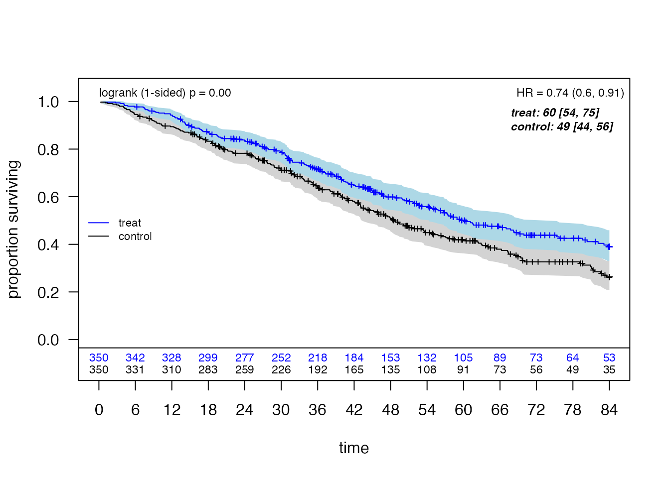

create_summary_table(
  data = sim_data, 
  treat_var = "treat", 
  table_title = "Characteristics by Treatment Arm",
  vars_continuous = c("z1", "z2", "size", "z3", "z4", "z5"),
  vars_categorical = c("flag.harm", "grade3"),
  font_size = 14
)

Characteristic		Control (n=350)	Treatment (n=350)	P-value¹	SMD²
Characteristics by Treatment Arm
z1	Mean (SD)	0.3 (0.4)	0.2 (0.4)	0.729	0.03
z2	Mean (SD)	2.4 (1.1)	2.5 (1.1)	0.157	0.11
size	Mean (SD)	29.2 (14.3)	30.1 (17.0)	0.461	0.06
z3	Mean (SD)	0.4 (0.5)	0.4 (0.5)	0.249	0.09
z4	Mean (SD)	2.6 (1.1)	2.5 (1.1)	0.428	0.06
z5	Mean (SD)	2.4 (1.1)	2.4 (1.1)	0.563	0.04
flag.harm				0.908	0.00
	0	306 (87.4%)	308 (88.0%)
	1	44 (12.6%)	42 (12.0%)
grade3				0.530	0.02
	0	273 (78.0%)	265 (75.7%)
	1	77 (22.0%)	85 (24.3%)
¹ P-values: t-test for continuous, chi-square/Fisher's exact for categorical/binary variables
² SMD = Standardized mean difference (Cohen's d for continuous, Cramer's V for categorical)

Running Simulation Studies

Setting Up Parallel Processing

For efficient simulation studies, use parallel processing:

# Configure parallel backend
n_workers <- min(parallel::detectCores() - 1, 120)

plan(multisession, workers = n_workers)

cat("Using", n_workers, "parallel workers\n")

## Using 13 parallel workers

Define Simulation Parameters

# Simulation settings
sim_config_alt <- list(
  n_sims = nsims_alt,          # Number of simulations (use 500-1000 for final)
  n_sample = 700,         # Sample size per trial
  max_follow = 84,        # Maximum follow-up (months)
  seed_base = 8316951,
  muC_adj = log(1.5)
)

sim_config_null <- list(
  n_sims = nsims_null,          # More simulations for Type I error estimation
  n_sample = 700,         # Sample size per trial
  max_follow = 84,        # Maximum follow-up (months)
  seed_base = 8316951,
  muC_adj = log(1.5)
)

# ForestSearch parameters (now includes use_twostage)
fs_params <- list(
  outcome.name = "y.sim",
  event.name = "event.sim",
  treat.name = "treat",
  id.name = "id",
  use_lasso = TRUE,
  use_grf = TRUE,
  hr.threshold = 1.25,
  hr.consistency = 1.0,
  pconsistency.threshold = 0.90,
  fs.splits = 400,
  n.min = 60,
  d0.min = 12,
  d1.min = 12,
  maxk = 2,
  by.risk = 12,
  vi.grf.min = -0.2,
  # NEW: Two-stage algorithm option
  use_twostage = TRUE,      # Set TRUE for faster exploratory analysis
  twostage_args = list()     # Optional tuning parameters
)


# Confounders for analysis
confounders_base <- c("z1", "z2", "z3", "z4", "z5", "size", "grade3")

Two-Stage Algorithm Option

The use_twostage parameter enables a faster two-stage search algorithm:

# Fast configuration with two-stage algorithm
fs_params_fast <- modifyList(fs_params, list(
  use_twostage = TRUE,
  twostage_args = list(
    n.splits.screen = 30,    # Stage 1 screening splits
    batch.size = 20,         # Stage 2 batch size
    conf.level = 0.95        # Early stopping confidence
  )
))

cat("Standard search: use_twostage =", fs_params$use_twostage, "\n")

## Standard search: use_twostage = TRUE

cat("Fast search: use_twostage =", fs_params_fast$use_twostage, "\n")

## Fast search: use_twostage = TRUE

Running Alternative Hypothesis Simulations

cat("Running", sim_config_alt$n_sims, "simulations under H1...\n")

## Running 1000 simulations under H1...

start_time <- Sys.time()
t0 <- proc.time()[3]

results_alt <- foreach(
  sim = 1:sim_config_alt$n_sims,
  .combine = rbind,
  .errorhandling = "remove",
  .options.future = list(
    packages = c("forestsearch", "survival", "data.table"),
    seed = TRUE
  )
) %dofuture% {
  run_simulation_analysis(
    sim_id = sim,
    dgm = dgm_calibrated,
    n_sample = sim_config_alt$n_sample,
    max_follow = sim_config_alt$max_follow,
    muC_adj = sim_config_alt$muC_adj,
    confounders_base = confounders_base,
    cox_formula_adj = survival::Surv(y.sim, event.sim) ~ treat + z1 + z2 + z3,
    n_add_noise = 0L,
    run_fs = TRUE,
    run_fs_grf = FALSE,
    run_grf = TRUE,
    fs_params = fs_params,
    verbose = TRUE,
    debug = FALSE,
    verbose_n = 1  # Only print first 1 simulations
  )
}

## 
## === Two-Stage Consistency Evaluation Enabled ===
## Stage 1 screening splits: 30 
## Maximum total splits: 400 
## Batch size: 20 
## ================================================
## 
## GRF stage for cut selection with dmin, tau = 12 0.6 
##   return_selected_cuts_only = TRUE: using cuts from selected tree only
## tau, maxdepth = 48.53742 2 
##    leaf.node control.mean control.size control.se depth
## 1          2        -5.33       520.00       1.11     1
## 2          3         1.02       180.00       2.32     1
## 11         4        -6.71       426.00       1.21     2
## 21         5         3.44       142.00       2.62     2
## 4          7        -7.11        78.00       3.18     2
## GRF subgroup NOT found
## GRF cuts identified: 0 
## # of continuous/categorical characteristics 4 3 
## Continuous characteristics: z2 z4 z5 size 
## Categorical characteristics: z1 z3 grade3 
## ## Prior to lasso: z2 z4 z5 size 
## #### Lasso selection results 
## 7 x 1 sparse Matrix of class "dgCMatrix"
##                 s0
## z1      0.28638272
## z2      .         
## z3      0.04573174
## z4     -0.34834939
## z5      0.45235142
## size    .         
## grade3  0.01493646
## Cox-LASSO selected: z1 z3 z4 z5 grade3 
## Cox-LASSO not selected: z2 size 
## ### End Lasso selection 
## ## After lasso: z4 z5 
## Default cuts included from Lasso: z4 <= mean(z4) z4 <= median(z4) z4 <= qlow(z4) z4 <= qhigh(z4) z5 <= mean(z5) z5 <= median(z5) z5 <= qlow(z5) z5 <= qhigh(z5) 
## Categorical after Lasso: z1 z3 grade3 
## Factors per GRF:  
## Initial GRF cuts included  
## Factors included per GRF (not in lasso)  
## 
## ===== CONSOLIDATED CUT EVALUATION (IMPROVED) =====
## Evaluating 10 cut expressions once and caching...
## Cut evaluation summary:
##   Total cuts:  10 
##   Valid cuts:  10 
##   Errors:  0 
## ✓ All 10 factors validated as 0/1
## ===== END CONSOLIDATED CUT EVALUATION =====
## 
## # of candidate subgroup factors= 10 
##  [1] "z4 <= 2.5" "z4 <= 3"   "z4 <= 2"   "z5 <= 2.4" "z5 <= 2"   "z5 <= 1"  
##  [7] "z5 <= 3"   "z1"        "z3"        "grade3"   
## Number of possible configurations (<= maxk): maxk = 2 , # combinations = 210 
## Events criteria: control >= 12 , treatment >= 12 
## Sample size criteria: n >= 60 
## Subgroup search completed in 0.01 minutes
## 
## --- Filtering Summary ---
##   Combinations evaluated: 210 
##   Passed variance check: 189 
##   Passed prevalence (>= 0.025 ): 189 
##   Passed redundancy check: 178 
##   Passed event counts (d0>= 12 , d1>= 12 ): 160 
##   Passed sample size (n>= 60 ): 158 
##   Cox model fit successfully: 158 
##   Passed HR threshold (>= 1.25 ): 3 
## -------------------------
## 
## Found 3 subgroup candidate(s)
## # of candidate subgroups (meeting all criteria) = 3 
## Random seed set to: 8316951 
## Two-stage parameters:
##   n.splits.screen: 30 
##   screen.threshold: 0.763 
##   batch.size: 20 
##   conf.level: 0.95 
## Removed 1 near-duplicate subgroups
## # of unique initial candidates: 2 
## # Restricting to top stop_Kgroups = 10 
## # of candidates to evaluate: 2 
## # Early stop threshold: 0.95 
## Parallel config: workers = 6 , batch_size = 1 
## Batch 1 / 2 : candidates 1 - 1 
## Batch 2 / 2 : candidates 2 - 2 
## Evaluated 2 of 2 candidates (complete) 
## 1 subgroups passed consistency threshold
## SG focus = hr 
## Seconds and minutes forestsearch overall = 8.45 0.1408 
## Consistency algorithm used: twostage 
## tau, maxdepth = 48.53742 2 
##    leaf.node control.mean control.size control.se depth
## 1          2        -5.33       520.00       1.11     1
## 2          3         1.02       180.00       2.32     1
## 11         4        -6.71       426.00       1.21     2
## 21         5         3.44       142.00       2.62     2
## 4          7        -7.11        78.00       3.18     2
## GRF subgroup NOT found

timings$sims_alt_elapsed <- proc.time()[3] - t0
runtime_alt <- difftime(Sys.time(), start_time, units = "mins")
timings$sims_alt_wall <- as.numeric(runtime_alt) * 60  # store in seconds
cat("Completed in", round(runtime_alt, 1), "minutes\n")

## Completed in 7.9 minutes

cat("Results:", nrow(results_alt), "rows\n")

## Results: 2000 rows

Running Null Hypothesis Simulations

cat("Running", sim_config_null$n_sims, "simulations under H0...\n")

## Running 5000 simulations under H0...

start_time <- Sys.time()
t0 <- proc.time()[3]

results_null <- foreach(
  sim = 1:sim_config_null$n_sims,
  .combine = rbind,
  .errorhandling = "remove",
  .options.future = list(
    packages = c("forestsearch", "survival", "data.table"),
    seed = TRUE
  )
) %dofuture% {
  
  run_simulation_analysis(
    sim_id = sim,
    dgm = dgm_null,
    n_sample = sim_config_null$n_sample,
    max_follow = sim_config_null$max_follow,
    muC_adj = sim_config_null$muC_adj,
    confounders_base = confounders_base,
    cox_formula_adj = survival::Surv(y.sim, event.sim) ~ treat + z1 + z2 + z3,
    n_add_noise = 0L,
    run_fs = TRUE,
    run_fs_grf = FALSE,
    run_grf = TRUE,
    fs_params = fs_params,
    verbose = TRUE,
    verbose_n = 1  # Only print first 1 simulations

  )
}

## 
## === Two-Stage Consistency Evaluation Enabled ===
## Stage 1 screening splits: 30 
## Maximum total splits: 400 
## Batch size: 20 
## ================================================
## 
## GRF stage for cut selection with dmin, tau = 12 0.6 
##   return_selected_cuts_only = TRUE: using cuts from selected tree only
## tau, maxdepth = 47.91247 2 
##   leaf.node control.mean control.size control.se depth
## 2         3        -4.78       695.00       1.00     1
## 1         4        -5.09       568.00       1.10     2
## GRF subgroup NOT found
## GRF cuts identified: 0 
## # of continuous/categorical characteristics 4 3 
## Continuous characteristics: z2 z4 z5 size 
## Categorical characteristics: z1 z3 grade3 
## ## Prior to lasso: z2 z4 z5 size 
## #### Lasso selection results 
## 7 x 1 sparse Matrix of class "dgCMatrix"
##                   s0
## z1      0.0078483334
## z2      0.0324623135
## z3      .           
## z4     -0.3338944143
## z5      0.4663620842
## size    0.0002302206
## grade3  .           
## Cox-LASSO selected: z1 z2 z4 z5 size 
## Cox-LASSO not selected: z3 grade3 
## ### End Lasso selection 
## ## After lasso: z2 z4 z5 size 
## Default cuts included from Lasso: z2 <= mean(z2) z2 <= median(z2) z2 <= qlow(z2) z2 <= qhigh(z2) z4 <= mean(z4) z4 <= median(z4) z4 <= qlow(z4) z4 <= qhigh(z4) z5 <= mean(z5) z5 <= median(z5) z5 <= qlow(z5) z5 <= qhigh(z5) size <= mean(size) size <= median(size) size <= qlow(size) size <= qhigh(size) 
## Categorical after Lasso: z1 
## Factors per GRF:  
## Initial GRF cuts included  
## Factors included per GRF (not in lasso)  
## 
## ===== CONSOLIDATED CUT EVALUATION (IMPROVED) =====
## Evaluating 15 cut expressions once and caching...
## Cut evaluation summary:
##   Total cuts:  15 
##   Valid cuts:  14 
##   Errors:  0 
## Dropping variables (cut only has 1 level): z2 <= 4 
## Total cuts after dropping invalid: 14
## ✓ All 14 factors validated as 0/1
## ===== END CONSOLIDATED CUT EVALUATION =====
## 
## # of candidate subgroup factors= 14 
##  [1] "z2 <= 2.5"    "z2 <= 2"      "z4 <= 2.5"    "z4 <= 3"      "z4 <= 2"     
##  [6] "z5 <= 2.4"    "z5 <= 2"      "z5 <= 1"      "z5 <= 3"      "size <= 29.1"
## [11] "size <= 25"   "size <= 20"   "size <= 35"   "z1"          
## Number of possible configurations (<= maxk): maxk = 2 , # combinations = 406 
## Events criteria: control >= 12 , treatment >= 12 
## Sample size criteria: n >= 60 
## Subgroup search completed in 0.03 minutes
## 
## --- Filtering Summary ---
##   Combinations evaluated: 406 
##   Passed variance check: 373 
##   Passed prevalence (>= 0.025 ): 373 
##   Passed redundancy check: 354 
##   Passed event counts (d0>= 12 , d1>= 12 ): 327 
##   Passed sample size (n>= 60 ): 316 
##   Cox model fit successfully: 316 
##   Passed HR threshold (>= 1.25 ): 4 
## -------------------------
## 
## Found 4 subgroup candidate(s)
## # of candidate subgroups (meeting all criteria) = 4 
## Random seed set to: 8316951 
## Two-stage parameters:
##   n.splits.screen: 30 
##   screen.threshold: 0.763 
##   batch.size: 20 
##   conf.level: 0.95 
## Removed 2 near-duplicate subgroups
## # of unique initial candidates: 2 
## # Restricting to top stop_Kgroups = 10 
## # of candidates to evaluate: 2 
## # Early stop threshold: 0.95 
## Parallel config: workers = 6 , batch_size = 1 
## Batch 1 / 2 : candidates 1 - 1 
## Batch 2 / 2 : candidates 2 - 2 
## Evaluated 2 of 2 candidates (complete) 
## No subgroups found meeting consistency threshold
## Seconds and minutes forestsearch overall = 8.245 0.1374 
## Consistency algorithm used: twostage 
## tau, maxdepth = 47.91247 2 
##   leaf.node control.mean control.size control.se depth
## 2         3        -4.78       695.00       1.00     1
## 1         4        -5.09       568.00       1.10     2
## GRF subgroup NOT found

timings$sims_null_elapsed <- proc.time()[3] - t0
runtime_null <- difftime(Sys.time(), start_time, units = "mins")
timings$sims_null_wall <- as.numeric(runtime_null) * 60
cat("Completed in", round(runtime_null, 1), "minutes\n")

## Completed in 35.6 minutes

Summarizing Results

Operating Characteristics Summary Under HTEs

t0 <- proc.time()[3]

format_oc_results(results_alt, metrics = c("detection","classification","cde_estimates"), digits = 2, digits_hr = 2,
                  title = "Identification properties (HTEs)", 
                  subtitle = sprintf("n = %d, %d simulations, HR(overall) = %.2f",
                     sim_config_alt$n_sample,
                     sim_config_alt$n_sims,
                     dgm_calibrated$hr_causal))

Method	Sims	Found	Classification				Controlled Direct Effects
Identification properties (HTEs)
n = 700, 1000 simulations, HR(overall) = 0.72
Method	Sims	Found	Sen	Spec	PPV	NPV	θ‡(H)	θ‡(Hᶜ)	θ‡(Ĥ)	θ‡(Ĥᶜ)
FS	1000	0.88	0.86	0.98	0.89	0.98	2.40	0.58	2.21	0.63
GRF	1000	0.75	0.89	0.97	0.84	0.98	2.40	0.58	2.11	0.62

# Check for AHR columns in results
ahr_cols <- grep("ahr", names(results_alt), value = TRUE)
cat("AHR columns in results:", paste(ahr_cols, collapse = ", "), "\n\n")

## AHR columns in results: ahr.H.true, ahr.Hc.true, ahr.H.hat, ahr.Hc.hat

if (length(ahr_cols) > 0) {
  # Summarize AHR estimates
  results_found <- results_alt[results_alt$any.H == 1 & results_alt$analysis == "FS", ]
  
  if (nrow(results_found) > 0 && "ahr.H.hat" %in% names(results_found)) {
    cat("AHR estimates (when subgroup found):\n")
    cat("  Mean AHR(H) estimated:", round(mean(results_found$ahr.H.hat, na.rm = TRUE), 3), "\n")
    cat("  Mean AHR(Hc) estimated:", round(mean(results_found$ahr.Hc.hat, na.rm = TRUE), 3), "\n")
    cat("  True AHR(H):", round(dgm_calibrated$AHR_H_true, 3), "\n")
    cat("  True AHR(Hc):", round(dgm_calibrated$AHR_Hc_true, 3), "\n")
  }
}

## AHR estimates (when subgroup found):
##   Mean AHR(H) estimated: 2.142 
##   Mean AHR(Hc) estimated: 0.602 
##   True AHR(H): 2.4 
##   True AHR(Hc): 0.585

build_estimation_table(
  results = results_alt,
  dgm = dgm_calibrated,
  analysis_method = "FS",
  subtitle = sprintf("n = %d, %d simulations, HR(overall) = %.2f",
  sim_config_alt$n_sample,
  sim_config_alt$n_sims,
  dgm_calibrated$hr_causal),
  font_size = 16
)

	Avg	SD	Min	Max	b‡ (%)	b† (%)
Estimation Properties
n = 700, 1000 simulations, HR(overall) = 0.72 (FS: 880/1000 (88%) estimable)
Ĥ: 880 estimable, avg \|Ĥ\| = 86, θ†(H) = 2, θ‡(H) = 2.4
θ̂(Ĥ)	2.31	0.63	1.32	8.16	-3.91	15.31
âhr(Ĥ)	2.14	0.47	0.58	2.40	NA	-10.76
θ‡(Ĥ)	2.21	0.38	0.58	2.40	NA	-7.96
Ĥᶜ: avg \|Ĥᶜ\| = 614, θ†(Hᶜ) = 0.66, θ‡(Hᶜ) = 0.58
θ̂(Ĥᶜ)	0.64	0.07	0.45	0.91	9.63	-3.04
âhr(Ĥᶜ)	0.60	0.03	0.58	0.72	NA	3.01
θ‡(Ĥᶜ)	0.63	0.08	0.58	0.93	NA	8.15
θ̂(Ĥ) = plugin Cox HR in identified subgroup; θ̂*(Ĥ) = bootstrap bias-corrected; âhr(Ĥ) = average hazard ratio in identified subgroup; b† = bias relative to marginal HR θ† (causal truth); θ‡(Ĥ) = controlled direct effect in identified subgroup; b‡ = bias relative to CDE θ‡

timings$summarize_alt <- proc.time()[3] - t0

Interpretation of estimated treatment effects

interpret_estimation_table(
  results_alt, dgm_calibrated,
  analysis_method = "FS",
  scenario = "alt"
)

Under the alternative hypothesis (true HR(H) = 2, true HR(Hc) = 0.66), 880 of 1000 simulations (88.0%) identified a subgroup using FS. The identified subgroup averaged 86 patients (complement: 614).

The naive Cox HR in the identified subgroup averaged 2.31 (SD = 0.63), corresponding to 15.3% relative bias versus the true HR(H) = 2. In the complement, the estimate averaged 0.64 (-3.0% bias vs. true HR(Hc) = 0.66).

Relative to the controlled direct effect (CDE) truth theta-ddagger(H) = 2.4, the naive plugin shows -3.9% relative bias.

The average hazard ratio (AHR) in the identified subgroup averaged 2.14 (-10.8% relative bias vs. true AHR(H) = 2.4); in the complement, 0.6 (3.0% bias vs. true AHR(Hc) = 0.58). The AHR shows attenuated bias relative to the Cox HR, consistent with AHR being a marginal rather than conditional estimand.

Operating Characteristics Under NULL (no HTEs)

t0 <- proc.time()[3]


format_oc_results(results_null, metrics = c("detection","classification","cde_estimates"), digits = 2, digits_hr = 2,
                  title = "Identification properties (under Null)", 
                  subtitle = sprintf("n = %d, %d simulations, HR(overall) = %.2f",
                   sim_config_null$n_sample,
                   sim_config_null$n_sims,
                   dgm_null$hr_causal))

Method	Sims	Found	Classification				Controlled Direct Effects
Identification properties (under Null)
n = 700, 5000 simulations, HR(overall) = 0.72
Method	Sims	Found	Sen	Spec	PPV	NPV	θ‡(H)	θ‡(Hᶜ)	θ‡(Ĥ)	θ‡(Ĥᶜ)
FS	5000	0.06	-	0.86	0.00	1.00	-	0.65	0.65	0.65
GRF	5000	0.06	-	0.89	0.00	1.00	-	0.65	0.65	0.65

# Check for AHR columns in results
ahr_cols <- grep("ahr", names(results_null), value = TRUE)
cat("AHR columns in results:", paste(ahr_cols, collapse = ", "), "\n\n")

## AHR columns in results: ahr.H.true, ahr.Hc.true, ahr.H.hat, ahr.Hc.hat

if (length(ahr_cols) > 0) {
  # Summarize AHR estimates
  results_found <- results_null[results_null$any.H == 1 & results_null$analysis == "FS", ]
  
  if (nrow(results_found) > 0 && "ahr.H.hat" %in% names(results_found)) {
    cat("AHR estimates (when subgroup found):\n")
    cat("  Mean AHR(H) estimated:", round(mean(results_found$ahr.H.hat, na.rm = TRUE), 3), "\n")
    cat("  Mean AHR(Hc) estimated:", round(mean(results_found$ahr.Hc.hat, na.rm = TRUE), 3), "\n")
    cat("  True AHR(H):", round(dgm_null$AHR_H_true, 3), "\n")
    cat("  True AHR(Hc):", round(dgm_null$AHR_Hc_true, 3), "\n")
  }
}

## AHR estimates (when subgroup found):
##   Mean AHR(H) estimated: 0.654 
##   Mean AHR(Hc) estimated: 0.654 
##   True AHR(H): NA 
##   True AHR(Hc): 0.654

build_estimation_table(
  results = results_null,
  dgm = dgm_null,
  analysis_method = "FS",
  subtitle = sprintf("n = %d, %d simulations, HR(overall) = %.2f",
  sim_config_null$n_sample,
  sim_config_null$n_sims,
  dgm_null$hr_causal),
  font_size = 16
)

	Avg	SD	Min	Max	b‡ (%)	b† (%)
Estimation Properties
n = 700, 5000 simulations, HR(overall) = 0.72 (FS: 296/5000 (6%) estimable)
Ĥ: 296 estimable, avg \|Ĥ\| = 99, θ†(H) = 0.72, θ‡(H) = 0.65
θ̂(Ĥ)	1.80	0.26	1.35	2.89	174.56	148.72
âhr(Ĥ)	0.65	0.00	0.65	0.65	NA	0.00
θ‡(Ĥ)	0.65	0.00	0.65	0.65	NA	0.00
Ĥᶜ: avg \|Ĥᶜ\| = 601, θ†(Hᶜ) = 0.72, θ‡(Hᶜ) = 0.65
θ̂(Ĥᶜ)	0.68	0.07	0.46	0.93	3.24	-6.47
âhr(Ĥᶜ)	0.65	0.00	0.65	0.65	NA	0.00
θ‡(Ĥᶜ)	0.65	0.00	0.65	0.65	NA	0.00
θ̂(Ĥ) = plugin Cox HR in identified subgroup; θ̂*(Ĥ) = bootstrap bias-corrected; âhr(Ĥ) = average hazard ratio in identified subgroup; b† = bias relative to marginal HR θ† (causal truth); θ‡(Ĥ) = controlled direct effect in identified subgroup; b‡ = bias relative to CDE θ‡

timings$summarize_null <- proc.time()[3] - t0

Interpretation of estimated treatment effects

interpret_estimation_table(
  results_null, dgm_null,
  analysis_method = "FS",
  scenario = "null"
)

Under the null hypothesis (true HR = 0.72 uniformly), 296 of 5000 simulations (5.9%) identified a subgroup using FS. This low detection rate confirms controlled type-I error. Among those 296 false detections, the identified subgroup averaged 99 patients.

The naive Cox HR in the identified subgroup averaged 1.8 (SD = 0.26), representing 148.7% relative bias above the true value of 0.72. This upward bias reflects selection: the algorithm identified whichever patients happened to look most like a harm subgroup by chance. In the complement, the Cox HR averaged 0.68 (-6.5% bias), showing the expected mirror effect where removing the worst-looking patients makes the remainder appear modestly better.

Relative to the controlled direct effect (CDE) truth theta-ddagger(H) = 0.65, the naive plugin shows 174.6% relative bias.

The average hazard ratio (AHR) in the identified subgroup averaged 0.65 (0.0% relative bias vs. true AHR(H) = 0.65); in the complement, 0.65 (0.0% bias vs. true AHR(Hc) = 0.65). The AHR shows attenuated bias relative to the Cox HR, consistent with AHR being a marginal rather than conditional estimand.

These results underscore that under the null, the few false detections produce highly biased estimates, reinforcing the need for bootstrap bias correction for any subgroup identified by a data-driven search.

Classification Rate Details

# ── Assemble scenario list from the current vignette results ─────────────
scenario_list <- list(
  null = list(
    results    = results_null,
    label      = "M",
    n_sample   = sim_config_null$n_sample,
    dgm        = dgm_null,
    hypothesis = "null"
  ),
  alt = list(
    results    = results_alt,
    label      = "M",
    n_sample   = sim_config_alt$n_sample,
    dgm        = dgm_calibrated,
    hypothesis = "alt"
  )
)

# ── Build and display the classification table ───────────────────────────
build_classification_table(
  scenario_results = scenario_list,
  analyses = sort(unique(c(
    unique(results_null$analysis),
    unique(results_alt$analysis)
  ))),
  digits = 2,
  font_size = 16,
  title = "Subgroup Identification and Classification Rates",
  n_sims = sim_config_alt$n_sims
)

	FS	GRF
Subgroup Identification and Classification Rates
Across 1,000 simulations per scenario
M Null: N=700, theta(ITT) = 0.72
any(H)	0.06	0.06
sens(Hc)	0.86	0.89
ppv(Hc)	1.00	1.00
avg\|H\|	99.00	78.00
M Alt: N=700, p_H=13%, theta(H)=2, theta(Hc)=0.66, theta(ITT)=0.72
any(H)	0.88	0.75
sens(H)	0.86	0.89
sens(Hc)	0.98	0.97
ppv(H)	0.89	0.84
ppv(Hc)	0.98	0.98
avg\|H\|	86.00	98.00

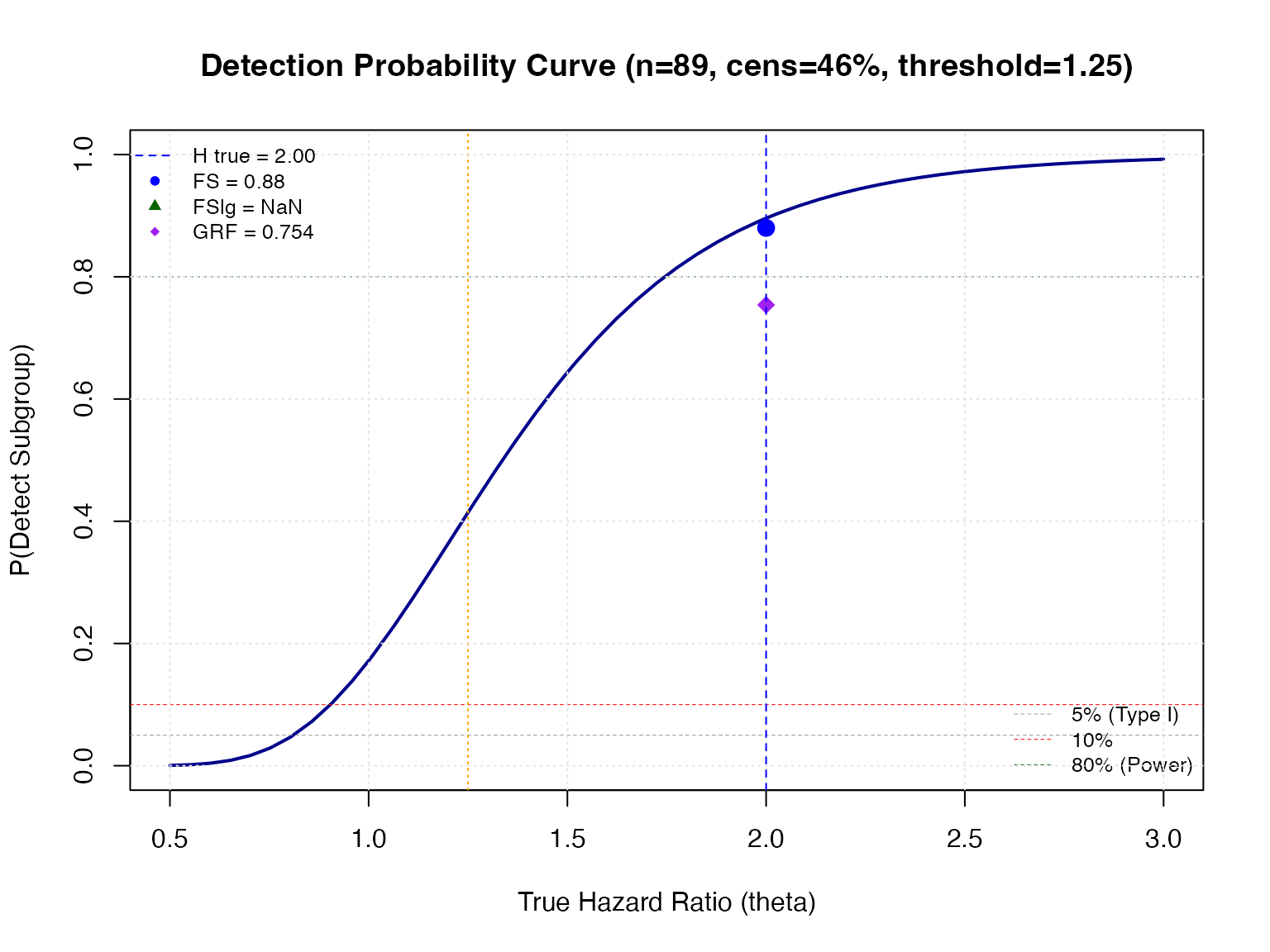
Theoretical Subgroup Detection Rate Approximation

The function compute_detection_probability() provides an analytical approximation based on asymptotic normal theory:

# =============================================================================
# Theoretical Detection Probability Analysis
# =============================================================================

# Calculate expected subgroup characteristics
n_sg_expected <- sim_config_alt$n_sample * mean(dgm_calibrated$df_super_rand$flag.harm)
prop_cens <- mean(results_alt$p.cens)  # Censoring proportion

cat("=== Subgroup Characteristics ===\n")

## === Subgroup Characteristics ===

cat("Expected subgroup size (n_sg):", round(n_sg_expected), "\n")

## Expected subgroup size (n_sg): 89

cat("Censoring proportion:", round(prop_cens, 3), "\n")

## Censoring proportion: 0.453

cat("True HR in H:", round(dgm_calibrated$hr_H_true, 3), "\n")

## True HR in H: 2

cat("HR threshold:", fs_params$hr.threshold, "\n")

## HR threshold: 1.25

# -----------------------------------------------------------------------------
# Single-Point Detection Probability
# -----------------------------------------------------------------------------

# True H is dgm_calibrated$hr_H_true
# However we want at plim of observed estimate
#plim_hr_hatH <- c(summary_alt[c("hat(hat[H])"),1])

dgm_calibrated$hr_H_true

##    treat 
## 1.999999

# Compute detection probability at the true HR
prob_detect <- compute_detection_probability(
 theta = dgm_calibrated$hr_H_true,
  n_sg = round(n_sg_expected),
  prop_cens = prop_cens,
  hr_threshold = fs_params$hr.threshold,
  hr_consistency = fs_params$hr.consistency,
  method = "cubature"
)

# Compare theoretical to empirical (alternative)
cat("\n=== Detection Probability Comparison ===\n")

## 
## === Detection Probability Comparison ===

cat("Theoretical FS (asymptotic):", round(prob_detect, 3), "\n")

## Theoretical FS (asymptotic): 0.899

cat("Empirical FS:", round(mean(results_alt[analysis == "FS"]$any.H), 3), "\n")

## Empirical FS: 0.88

cat("Empirical FSlg:", round(mean(results_alt[analysis == "FSlg"]$any.H), 3), "\n")

## Empirical FSlg: NaN

if ("GRF" %in% results_alt$analysis) {
  cat("Empirical GRF:", round(mean(results_alt[analysis == "GRF"]$any.H), 3), "\n")
}

## Empirical GRF: 0.754

# Null 

#plim_hr_itt <- c(summary_alt[c("hat(ITT)all"),1])

# Calculate at min SG size
# Compute detection probability at the true HR
prob_detect_null <- compute_detection_probability(
 theta = dgm_null$hr_causal,
  n_sg = fs_params$n.min,
  prop_cens = prop_cens,
  hr_threshold = fs_params$hr.threshold,
  hr_consistency = fs_params$hr.consistency,
  method = "cubature"
)


# Compare theoretical to empirical (alternative)
cat("\n=== Detection Probability Comparison ===\n")

## 
## === Detection Probability Comparison ===

cat("Under the null calculate at min SG size:", fs_params$n.min,"\n")

## Under the null calculate at min SG size: 60

cat("Theoretical FS at min(SG) (asymptotic):", round(prob_detect_null, 6), "\n")

## Theoretical FS at min(SG) (asymptotic): 0.039618

cat("Empirical FS:", round(mean(results_null[analysis == "FS"]$any.H), 6), "\n")

## Empirical FS: 0.0592

cat("Empirical FSlg:", round(mean(results_null[analysis == "FSlg"]$any.H), 6), "\n")

## Empirical FSlg: NaN

if ("GRF" %in% results_null$analysis) {
  cat("Empirical GRF:", round(mean(results_null[analysis == "GRF"]$any.H), 6), "\n")
}

## Empirical GRF: 0.0648

prop_cens <- mean(results_null$p.cens)  # Censoring proportion
cat("Censoring proportion:", round(prop_cens, 3), "\n")

## Censoring proportion: 0.463

# -----------------------------------------------------------------------------
# Generate Full Detection Curve
# -----------------------------------------------------------------------------

# Generate detection probability curve across HR values
detection_curve <- generate_detection_curve(
  theta_range = c(0.5, 3.0),
  n_points = 50,
  n_sg = round(n_sg_expected),
  prop_cens = prop_cens,
  hr_threshold = fs_params$hr.threshold,
  hr_consistency = fs_params$hr.consistency,
  include_reference = TRUE,
  verbose = FALSE
)

# -----------------------------------------------------------------------------
# Visualization
# -----------------------------------------------------------------------------

# Plot detection curve with empirical overlay
plot_detection_curve(
  detection_curve,
  add_reference_lines = TRUE,
  add_threshold_line = TRUE,
  title = sprintf(
    "Detection Probability Curve (n=%d, cens=%.0f%%, threshold=%.2f)",
    round(n_sg_expected), 100 * prop_cens, fs_params$hr.threshold
  )
)

# Add empirical results as points
empirical_rates <- c(
  FS = mean(results_alt[analysis == "FS"]$any.H),
  FSlg = mean(results_alt[analysis == "FSlg"]$any.H)
)
if ("GRF" %in% results_alt$analysis) {
  empirical_rates["GRF"] <- mean(results_alt[analysis == "GRF"]$any.H)
}

# Mark the true HR and empirical detection rates
points(
  x = rep(dgm_calibrated$hr_H_true, length(empirical_rates)),
  y = empirical_rates,
  pch = c(16, 17, 18)[1:length(empirical_rates)],
  col = c("blue", "darkgreen", "purple")[1:length(empirical_rates)],
  cex = 1.5
)

# Add vertical line at true HR
abline(v = dgm_calibrated$hr_H_true, lty = 2, col = "blue", lwd = 1)

# Legend for empirical points
legend(
  "topleft",
  legend = c(
    sprintf("H true = %.2f", dgm_calibrated$hr_H_true),
    paste(names(empirical_rates), "=", round(empirical_rates, 3))
  ),
  pch = c(NA, 16, 17, 18)[1:(length(empirical_rates) + 1)],
  lty = c(2, rep(NA, length(empirical_rates))),
  col = c("blue", "blue", "darkgreen", "purple")[1:(length(empirical_rates) + 1)],
  cex = 0.8,
  bty = "n"
)

# Format operating characteristics for H0
format_oc_results(
  results = results_null,
  title = "Type I Error (Null Hypothesis)",
  subtitle = sprintf("n = %d, %d simulations, HR(overall) = %.2f",
                     sim_config_null$n_sample,
                     sim_config_null$n_sims,
                     dgm_null$hr_causal),
  use_gt = TRUE
)

Method	Sims	Found	Classification				Cox Hazard Ratios					Average Hazard Ratios				Controlled Direct Effects				Size_H_mean	Size_H_min	Size_H_max
Type I Error (Null Hypothesis)
n = 700, 5000 simulations, HR(overall) = 0.72
Method	Sims	Found	Sen	Spec	PPV	NPV	θ̂(Ĥ)	θ̂(Ĥᶜ)	θ̂(H)	θ̂(Hᶜ)	θ̂(ITT)	âhr(H)	âhr(Hᶜ)	âhr(Ĥ)	âhr(Ĥᶜ)	θ‡(H)	θ‡(Hᶜ)	θ‡(Ĥ)	θ‡(Ĥᶜ)	Size_H_mean	Size_H_min	Size_H_max
FS	5000	0.059	-	0.859	0.000	1.000	1.796	0.676	-	0.766	0.698	-	0.654	0.654	0.654	-	0.654	0.654	0.654	99	61	386
GRF	5000	0.065	-	0.888	0.000	1.000	1.524	0.666	-	-	0.698	-	0.654	0.654	0.654	-	0.654	0.654	0.654	78	60	177

Key Metrics

# Extract key metrics
cat("=== KEY OPERATING CHARACTERISTICS ===\n\n")

## === KEY OPERATING CHARACTERISTICS ===

cat("Alternative Hypothesis (H1):\n")

## Alternative Hypothesis (H1):

for (analysis in unique(results_alt$analysis)) {
  res <- results_alt[results_alt$analysis == analysis, ]
  cat(sprintf("  %s: Power = %.3f, Sens = %.3f, Spec = %.3f, PPV = %.3f\n",
              analysis,
              mean(res$any.H),
              mean(res$sens, na.rm = TRUE),
              mean(res$spec, na.rm = TRUE),
              mean(res$ppv, na.rm = TRUE)))
}

##   FS: Power = 0.817, Sens = 0.875, Spec = 0.978, PPV = 0.870
##   GRF: Power = 0.817, Sens = 0.875, Spec = 0.978, PPV = 0.870

cat("\nNull Hypothesis (H0):\n")

## 
## Null Hypothesis (H0):

for (analysis in unique(results_null$analysis)) {
  res <- results_null[results_null$analysis == analysis, ]
  cat(sprintf("  %s: Type I Error = %.4f\n",
              analysis,
              mean(res$any.H)))
}

##   FS: Type I Error = 0.0620
##   GRF: Type I Error = 0.0620

Using `format_oc_results()`

The format_oc_results() function is a flexible tool for creating publication-quality tables from simulation results. It accepts the raw data.table produced by run_simulation_analysis() (or combined via rbind / rbindlist across simulations) and returns either a gt table object or a plain data.frame.

Function Signature

format_oc_results(
  results,
  analyses = NULL,
  metrics = "all",
  digits = 3,
  digits_hr = 3,
  title = "Operating Characteristics Summary",
  subtitle = NULL,
  use_gt = TRUE
)

Key Parameters

Parameter	Default	Description
`results`	(required)	A `data.table` or `data.frame` with columns `analysis`, `any.H`, `sens`, `spec`, `ppv`, `npv`, `hr.H.hat`, etc., as produced by `run_simulation_analysis()`.
`analyses`	`NULL`	Character vector of analysis labels to include, e.g., `c("FS", "FSlg", "GRF")`. When `NULL`, all unique values of `results$analysis` are included.
`metrics`	`"all"`	Which metric groups to show: `"detection"`, `"classification"`, `"hr_estimates"`, `"subgroup_size"`, or `"all"`.
`digits`	`3`	Decimal places for proportions (detection rate, sens, spec, PPV, NPV).
`digits_hr`	`3`	Decimal places for hazard ratio estimates.
`title`	`"Operating Characteristics Summary"`	Table title shown in the `gt` header.
`subtitle`	`NULL`	Optional subtitle (e.g., sample size and true HR).
`use_gt`	`TRUE`	If `TRUE` and the `gt` package is available, returns a styled `gt` table; otherwise returns a `data.frame`.

Output Structure

When metrics = "all", the returned table contains one row per analysis method with the following columns:

Column	Description
`Detection`	Proportion of simulations that identified any subgroup (`any.H`)
`Sen`	Mean sensitivity across all simulations
`Spec`	Mean specificity
`PPV`	Mean positive predictive value
`NPV`	Mean negative predictive value
`HR_H_hat`	Mean estimated HR in identified subgroup (when found)
`HR_Hc_hat`	Mean estimated HR in complement (when found)
`HR_ITT`	Mean overall (ITT) HR across all simulations
`Size_H_mean`	Mean size of identified subgroup (when found)

Usage Patterns

Pattern 1: Quick summary of a single simulation run

# After running simulations
format_oc_results(results_alt, title = "H1 Results")

Pattern 2: Compare specific analysis methods

# Compare only FS and GRF
format_oc_results(
  results_alt,
  analyses = c("FS", "GRF"),
  title = "FS vs GRF Comparison"
)

Pattern 3: Focus on classification metrics only

format_oc_results(
  results_alt,
  metrics = "classification",
  title = "Classification Performance"
)

Pattern 4: Extract as data.frame for custom processing

# Get raw summary data.frame for further manipulation
oc_df <- format_oc_results(results_alt, use_gt = FALSE)

# Use for custom plotting or LaTeX export

Pattern 5: Multiple scenarios side-by-side

# Create tables for different sample sizes or HR targets
for (scenario in names(results_list)) {
  cat("\n", scenario, "\n")
  print(format_oc_results(
    results_list[[scenario]],
    title = scenario,
    subtitle = sprintf("n = %d", sample_sizes[[scenario]])
  ))
}

Pattern 6: Combine with summarize_simulation_results() for detailed output

summarize_simulation_results() returns a data.frame with row names like any.H, sens, spec, etc. (from summarize_single_analysis()), and one column per analysis method. This is useful for programmatic access to the raw summary statistics, while format_oc_results() is oriented toward presentation-quality tables:

# Detailed numeric summary (for computation)
summary_df <- summarize_simulation_results(results_alt)

# Presentation table (for reports)
format_oc_results(results_alt, title = "Publication Table")

Advanced Topics

Comparing Standard vs Two-Stage Algorithm

# Run simulations with two-stage algorithm for comparison
results_twostage <- foreach(
  sim = 1:100,
  .combine = rbind,
  .options.future = list(
    packages = c("forestsearch", "survival", "data.table"),
    seed = TRUE
  )
) %dofuture% {
  
  run_simulation_analysis(
    sim_id = sim,
    dgm = dgm_calibrated,
    n_sample = sim_config_alt$n_sample,
    confounders_base = confounders_base,
    run_fs = TRUE,
    run_fs_grf = FALSE,
    run_grf = FALSE,
    fs_params = fs_params_fast,  # use_twostage = TRUE
    verbose = FALSE
  )
}

# Compare detection rates
cat("Standard algorithm power:", round(mean(results_alt$any.H[results_alt$analysis == "FS"]), 3), "\n")
cat("Two-stage algorithm power:", round(mean(results_twostage$any.H), 3), "\n")

Adding Noise Variables

Test ForestSearch robustness by including irrelevant noise variables:

# Run simulations with noise variables
results_noise <- foreach(
  sim = 1:sim_config_alt$n_sims,
  .combine = rbind,
  .errorhandling = "remove",
  .options.future = list(
    packages = c("forestsearch", "survival", "data.table"),
    seed = TRUE
  )
) %dofuture% {
  
  run_simulation_analysis(
    sim_id = sim,
    dgm = dgm_calibrated,
    n_sample = sim_config_alt$n_sample,
    confounders_base = confounders_base,
    n_add_noise = 10,  # Add 10 noise variables
    run_fs = TRUE,
    fs_params = fs_params,
    verbose = FALSE
  )
}

# Compare detection rates
cat("Without noise:", round(mean(results_alt$any.H), 3), "\n")
cat("With 10 noise vars:", round(mean(results_noise$any.H), 3), "\n")

Sensitivity Analysis: Varying Parameters

# Test different HR thresholds
thresholds <- c(1.10, 1.25, 1.50)
results_by_thresh <- list()

for (thresh in thresholds) {
  results_by_thresh[[as.character(thresh)]] <- foreach(
    sim = 1:100,
    .combine = rbind,
    .options.future = list(
      packages = c("forestsearch", "survival", "data.table"),
      seed = TRUE
    )
  ) %dofuture% {
    
    run_simulation_analysis(
      sim_id = sim,
      dgm = dgm_calibrated,
      n_sample = sim_config_alt$n_sample,
      confounders_base = confounders_base,
      run_fs = TRUE,
      fs_params = modifyList(fs_params, list(hr.threshold = thresh)),
      verbose = FALSE
    )
  }
  results_by_thresh[[as.character(thresh)]]$threshold <- thresh
}

# Combine and summarize
combined <- rbindlist(results_by_thresh)
combined[, .(power = mean(any.H), ppv = mean(ppv, na.rm = TRUE)), 
         by = .(threshold, analysis)]

Saving Results

# Save simulation results for later use
save_simulation_results(
  results = results_alt,
  dgm = dgm_calibrated,
  summary_table = summary_alt,
  runtime_hours = as.numeric(runtime_alt) / 60,
  output_file = "forestsearch_simulation_alt.Rdata",
  # Include AHR metrics in saved output
  ahr_metrics = list(
    AHR_H_true = dgm_calibrated$AHR_H_true,
    AHR_Hc_true = dgm_calibrated$AHR_Hc_true,
    AHR = dgm_calibrated$AHR
  )
)

save_simulation_results(
  results = results_null,
  dgm = dgm_null,
  summary_table = summary_null,
  runtime_hours = as.numeric(runtime_null) / 60,
  output_file = "forestsearch_simulation_null.Rdata"
)

Computational Timing Summary

Tracking wall-clock time for every stage of a simulation study is essential for planning larger experiments and for reporting reproducibility information.

Stage	Time (sec)¹	Time (min)	% of Total
Computational Timing Summary
1000 H1 + 5000 H0 simulations, 13 workers
DGM creation (H1)	0.0	0.00	0.0
Calibrate k_inter (Cox)	2.0	0.03	0.1
Calibrate k_inter (AHR)	0.9	0.02	0.0
Validate k_inter	0.2	0.00	0.0
DGM creation (H0)	0.0	0.00	0.0
Simulations H1	475.3	7.92	18.0
Simulations H0	2,138.6	35.64	81.2
Summarize H1	0.1	0.00	0.0
Summarize H0	0.1	0.00	0.0
Total vignette	2,633.7	43.89	100.0
¹ Parallel backend: 13 workers via future::multisession.

Code

# Finalize total vignette time
timings$total <- (proc.time() - t_vignette_start)["elapsed"]

# ── Build timing data.frame ─────────────────────────────────────────────────
timing_df <- data.frame(
  Stage = c(
    "DGM creation (H1)",
    "Calibrate k_inter (Cox)",
    "Calibrate k_inter (AHR)",
    "Validate k_inter",
    "DGM creation (H0)",
    "Simulations H1",
    "Simulations H0",
    "Summarize H1",
    "Summarize H0",
    "Total vignette"
  ),
  Seconds = c(
    timings$dgm_creation,
    timings$calibrate_cox,
    timings$calibrate_ahr,
    timings$validation,
    timings$dgm_null,
    timings$sims_alt_elapsed,
    timings$sims_null_elapsed,
    timings$summarize_alt,
    timings$summarize_null,
    timings$total
  ),
  stringsAsFactors = FALSE
)

timing_df$Minutes <- timing_df$Seconds / 60
timing_df$Pct <- 100 * timing_df$Seconds / timings$total

# ── Present as gt table ─────────────────────────────────────────────────────
gt(timing_df) |>
  tab_header(
    title = "Computational Timing Summary",
    subtitle = sprintf(
      "%d H1 + %d H0 simulations, %d workers",
      sim_config_alt$n_sims,
      sim_config_null$n_sims,
      n_workers
    )
  ) |>
  fmt_number(columns = Seconds, decimals = 1) |>
  fmt_number(columns = Minutes, decimals = 2) |>
  fmt_number(columns = Pct, decimals = 1) |>
  cols_label(
    Stage   = "Stage",
    Seconds = "Time (sec)",
    Minutes = "Time (min)",
    Pct     = "% of Total"
  ) |>
  tab_style(
    style = cell_text(weight = "bold"),
    locations = cells_body(rows = Stage == "Total vignette")
  ) |>
  tab_footnote(
    footnote = sprintf("Parallel backend: %d workers via future::multisession.",
                       n_workers),
    locations = cells_column_labels(columns = Seconds)
  )

Per-Simulation Timing

If per-simulation timing is available in the results (via a time_elapsed column or similar), it can be summarized to characterize the distribution of runtimes across individual simulations:

# If run_simulation_analysis() stored per-sim elapsed time:
if ("time_elapsed" %in% names(results_alt)) {
  per_sim_stats <- results_alt[
    , .(
      mean_sec  = mean(time_elapsed, na.rm = TRUE),
      median_sec = median(time_elapsed, na.rm = TRUE),
      sd_sec    = sd(time_elapsed, na.rm = TRUE),
      min_sec   = min(time_elapsed, na.rm = TRUE),
      max_sec   = max(time_elapsed, na.rm = TRUE)
    ),
    by = analysis
  ]
  
  gt(per_sim_stats) |>
    tab_header(title = "Per-Simulation Timing (seconds)") |>
    fmt_number(columns = 2:6, decimals = 1)
}

Alternatively, the overall wall-clock time divided by the number of simulations gives the effective per-simulation cost accounting for parallel overhead:

cat("Effective per-simulation cost:\n")

## Effective per-simulation cost:

cat(sprintf("  H1: %.1f sec/sim (wall) across %d sims on %d workers\n",
            timings$sims_alt_elapsed / sim_config_alt$n_sims,
            sim_config_alt$n_sims, n_workers))

##   H1: 0.5 sec/sim (wall) across 1000 sims on 13 workers

cat(sprintf("  H0: %.1f sec/sim (wall) across %d sims on %d workers\n",
            timings$sims_null_elapsed / sim_config_null$n_sims,
            sim_config_null$n_sims, n_workers))

##   H0: 0.4 sec/sim (wall) across 5000 sims on 13 workers

Complete Example Script

Here’s a minimal self-contained script for running a simulation study:

# ===========================================================================
# Complete ForestSearch Simulation Study - Minimal Example (Aligned)
# ===========================================================================

library(forestsearch)
library(data.table)
library(survival)
library(foreach)
library(doFuture)

# --- Configuration ---
N_SIMS <- 500
N_SAMPLE <- 500
TARGET_HR_HARM <- 1.5

# --- Setup parallel processing ---
plan(multisession, workers = 4)

# --- Create DGM ---
# Option 1: Calibrate to Cox-based HR
k_inter <- calibrate_k_inter(target_hr_harm = TARGET_HR_HARM, 
                             use_ahr = FALSE, verbose = TRUE)

# Option 2: Calibrate to AHR instead
# k_inter <- calibrate_k_inter(target_hr_harm = TARGET_HR_HARM, 
#                              use_ahr = TRUE, verbose = TRUE)

dgm <- create_gbsg_dgm(model = "alt", k_inter = k_inter, verbose = TRUE)

# Verify hazard ratios (new aligned output)
cat("\nDGM Summary:\n")
cat("  Cox HR(H):", round(dgm$hr_H_true, 3), "\n")
cat("  AHR(H):", round(dgm$AHR_H_true, 3), "\n")
cat("  Cox HR(Hc):", round(dgm$hr_Hc_true, 3), "\n")
cat("  AHR(Hc):", round(dgm$AHR_Hc_true, 3), "\n")

# --- Run simulations ---
confounders <- c("v1", "v2", "v3", "v4", "v5", "v6", "v7")

results <- foreach(
  sim = 1:N_SIMS, 
  .combine = rbind,
  .options.future = list(
    packages = c("forestsearch", "survival", "data.table"),
    seed = TRUE
  )
) %dofuture% {
  run_simulation_analysis(
    sim_id = sim,
    dgm = dgm,
    n_sample = N_SAMPLE,
    max_follow = 60,
    confounders_base = confounders,
    run_fs = TRUE,
    run_fs_grf = TRUE,
    run_grf = FALSE,
    fs_params = list(
      hr.threshold = 1.25, 
      fs.splits = 300, 
      maxk = 2,
      use_twostage = FALSE  # Set TRUE for faster analysis
    )
  )
}

# --- Summarize ---
summary_table <- summarize_simulation_results(results)
print(summary_table)

# --- Display formatted table ---
format_oc_results(results = results, title = sprintf("Operating Characteristics (n=%d)", N_SAMPLE))

# --- Report AHR metrics (new) ---
results_found <- results[results$any.H == 1, ]
if (nrow(results_found) > 0 && "ahr.H.hat" %in% names(results_found)) {
  cat("\nAHR Estimates:\n")
  cat("  True AHR(H):", round(dgm$AHR_H_true, 3), "\n")
  cat("  Mean estimated AHR(H):", round(mean(results_found$ahr.H.hat, na.rm = TRUE), 3), "\n")
}

Summary

This vignette demonstrated the complete workflow for evaluating ForestSearch performance through simulation:

Step	Function	Purpose
1. Create DGM	`create_gbsg_dgm()`	Define data generating mechanism
2. Calibrate	`calibrate_k_inter()`	Achieve target subgroup HR (Cox or AHR)
3. Validate	`validate_k_inter_effect()`	Verify heterogeneity control
4. Simulate	`simulate_from_gbsg_dgm()`	Generate trial data
5. Analyze	`run_simulation_analysis()`	Run ForestSearch/GRF
6. Summarize	`summarize_simulation_results()`	Aggregate metrics
7. Display	`format_oc_results()`	Create gt tables

Key metrics to report:

Power (H1) / Type I Error (H0): Subgroup detection rate
Sensitivity: P(identified | true harm subgroup)
Specificity: P(not identified | true complement)
PPV: P(true harm | identified)
NPV: P(true complement | not identified)

New aligned features:

AHR metrics: Alternative to Cox-based HR (from loghr_po)
use_ahr calibration: Calibrate to AHR instead of Cox HR
use_twostage: Faster two-stage search algorithm option
Individual effects: Access theta_0, theta_1, loghr_po per subject

Appendix A: Publication-Quality Tables

This appendix demonstrates how to build publication-quality tables from summarize_simulation_results() output that match the structure and content of the tables in Leon et al. (2024). The two target table formats are:

Table 1 (Classification): Subgroup identification and classification rates across multiple data generation scenarios and analysis methods (cf. Table 4 of Leon et al.).
Table 2 (Estimation): Estimation properties including bias, coverage, and confidence interval metrics for the identified subgroup hazard ratios.

Package Functions for Table Construction

The forestsearch package provides three exported functions for building publication-quality simulation tables. These are defined in R/simulation_tables.R and available after loading the package:

build_classification_table(): Constructs a grouped gt table of subgroup identification and classification rates across scenarios, matching the layout of Table 4 in Leon et al. (2024).
build_estimation_table(): Summarizes estimation properties (Avg, SD, Min, Max, relative bias) for HR estimates in identified subgroups, matching Table 5 of Leon et al. (2024). When CDE values are available (from the DGM or supplied explicitly via cde_H/cde_Hc), produces dual bias columns: b‡ (vs CDE θ‡) and b† (vs marginal HR θ†).
render_reference_table(): Renders a pre-assembled data frame of reference results as a styled gt table with consistent formatting.

See ?build_classification_table, ?build_estimation_table, and ?render_reference_table for full documentation.

Generating Tables from Current Simulation Results

Using the package table functions, we construct tables from the simulation results obtained in this vignette. These demonstrate the table format; for a full replication of the Leon et al. (2024) tables, one would run multiple scenarios (e.g., M1: N=700, M2: N=500, M3: N=300) with 20,000 simulations each.

Table 1: Classification Rates

This is a repeat from above (do not run)

# ── Assemble scenario list from the current vignette results ─────────────
scenario_list <- list(
  null = list(
    results    = results_null,
    label      = "M",
    n_sample   = sim_config_null$n_sample,
    dgm        = dgm_null,
    hypothesis = "null"
  ),
  alt = list(
    results    = results_alt,
    label      = "M",
    n_sample   = sim_config_alt$n_sample,
    dgm        = dgm_calibrated,
    hypothesis = "alt"
  )
)

# ── Build and display the classification table ───────────────────────────
build_classification_table(
  scenario_results = scenario_list,
  analyses = sort(unique(c(
    unique(results_null$analysis),
    unique(results_alt$analysis)
  ))),
  digits = 2,
  title = "Subgroup Identification and Classification Rates",
  n_sims = sim_config_alt$n_sims
)

Table 2: Estimation Properties

Not run (duplicate of above).

Detailed calculations follow.

# ── Build estimation table for the preferred analysis method ──────────────
# Uses the alternative-hypothesis results where subgroups are identified.
# If "FSlg" is not present, fall back to "FS".
# CDE values are auto-extracted from the DGM via get_dgm_hr().
# When CDE is available, dual bias columns b‡ (CDE) and b† (marginal) appear.

est_analysis <- if ("FSlg" %in% unique(results_alt$analysis)) "FSlg" else "FS"

build_estimation_table(
  results = results_alt,
  dgm     = dgm_calibrated,
  analysis_method = est_analysis,
  digits  = 2,
  title   = "Estimation Properties for Identified Subgroup"
)

Detailed Summary: How `build_estimation_table()` Calculates Results

`R/simulation_tables.R`

Purpose

build_estimation_table() produces a gt table summarizing how well ForestSearch (or GRF) estimates the treatment-effect hazard ratio in the identified subgroup (Ĥ) and its complement (Ĥᶜ). It reports average estimate, variability, range, and relative bias versus DGM truth for up to eight estimators across two row-groups. When CDE (controlled direct effect) values are available, dual bias columns are shown: b‡ (relative to CDE θ‡) and b† (relative to marginal HR θ†), aligning with Table 5 of Leon et al. (2024).

Input Requirements

Argument	Role
`results`	`data.table` from `run_simulation_analysis()`, one row per sim × method
`dgm`	DGM object carrying true parameter values
`analysis_method`	Which method to filter on (e.g., `"FS"`, `"FSlg"`, `"GRF"`)
`n_boots`	Optional; if non-NULL, shown in subtitle
`cde_H`	Optional CDE for harm subgroup (θ‡(H)); auto-extracted from DGM if NULL
`cde_Hc`	Optional CDE for complement (θ‡(Hᶜ)); auto-extracted from DGM if NULL
`digits`	Rounding precision for all displayed numbers
`font_size`	Pixel size for gt rendering

Step-by-Step Calculation Pipeline

1. Filter to Estimable Realizations

res <- as.data.table(results)
res <- res[analysis == analysis_method]   # keep only the requested method
res_found <- res[any.H == 1]             # keep only sims that found a subgroup
n_estimable <- nrow(res_found)

Only simulations where the algorithm identified a subgroup (any.H == 1) contribute to estimation summaries. If n_estimable == 0, the function returns NULL with a message.

2. Extract True Values from the DGM

Alternative hypothesis DGM (model = "alt"):

True value	Source	Description
`theta_H_true`	`dgm$hr_H_true`	Cox-based HR in the true harm subgroup
`theta_Hc_true`	`dgm$hr_Hc_true`	Cox-based HR in the true complement
`ahr_H_true`	`get_dgm_hr(dgm, "ahr_H")`	AHR in the true harm subgroup
`ahr_Hc_true`	`get_dgm_hr(dgm, "ahr_Hc")`	AHR in the true complement
`cde_H`	`get_dgm_hr(dgm, "cde_H")`	CDE in harm subgroup (θ‡(H))
`cde_Hc`	`get_dgm_hr(dgm, "cde_Hc")`	CDE in complement (θ‡(Hᶜ))

CDE auto-detection: When cde_H and cde_Hc are not supplied by the caller, the function attempts to extract them from the DGM via get_dgm_hr(). If that fails but the DGM contains a super-population with theta_0 and theta_1 columns, compute_dgm_cde() is called as a fallback to compute and attach CDE values. Under the null hypothesis, if only an overall CDE is available (get_dgm_hr(dgm, "cde")), it is used for both subgroups (since the treatment effect is uniform). When CDE values are present, the table produces dual bias columns: b‡ (relative to CDE) and b† (relative to marginal HR), matching Table 5 of Leon et al. (2024).

Null hypothesis DGM (model = "null"):

Under the null, hr_H_true is NA because no true subgroup exists. The function detects this via:

is_null <- (dgm$model_type == "null") ||
           (is.na(theta_H_true) && !is.na(theta_Hc_true))

When is_null is TRUE, all NA true values are backfilled with the overall (causal) HR, which is the uniform true value for any subset:

hr_overall  <- get_dgm_hr(dgm, "hr_overall")  # tries hazard_ratios$overall
if (is.na(hr_overall)) hr_overall <- dgm$hr_causal  # fallback to direct field

theta_H_true  <- hr_overall   # e.g., 0.72
theta_Hc_true <- hr_overall   # same value under the null

The same logic applies for AHR via get_dgm_hr(dgm, "ahr") / dgm$AHR.

3. Compute Per-Estimator Summary Statistics

The core computation is handled by the make_est_row() helper:

make_est_row <- function(estimates, true_val, label, cde_val = NA_real_) {
  est <- estimates[!is.na(estimates)]   # drop any NA estimates
  if (length(est) == 0) return(NULL)

  avg_est  <- mean(est)
  sd_est   <- sd(est)
  min_est  <- min(est)
  max_est  <- max(est)

  # b-dagger: bias relative to marginal (causal) truth
  b_dagger <- 100 * (avg_est - true_val) / true_val

  row <- data.frame(
    Estimator    = label,
    Avg          = round(avg_est, digits),
    SD           = round(sd_est, digits),
    Min          = round(min_est, digits),
    Max          = round(max_est, digits)
  )

  if (has_cde && !is.na(cde_val)) {
    # b-ddagger: bias relative to CDE truth
    b_ddagger <- 100 * (avg_est - cde_val) / cde_val
    row[["b-ddagger (%)"]] <- round(b_ddagger, digits)
    row[["b-dagger (%)"]]  <- round(b_dagger, digits)
  } else {
    row[["b-dagger (%)"]]  <- round(b_dagger, digits)
  }
  row
}

Key formulas — Relative Bias:

b† (%)  = 100 * (mean(theta-hat) - theta†) / theta†     [marginal truth]
b‡ (%)  = 100 * (mean(theta-hat) - theta‡) / theta‡     [CDE truth]

The b† column always appears; it measures percentage bias versus the DGM’s marginal/causal HR (θ†). When CDE values are available, a second column b‡ is prepended, measuring bias versus the controlled direct effect (θ‡). This dual-column layout matches the Bias_dagger / Bias_ddagger columns in Table 5 of Leon et al. (2024). Positive values indicate upward bias (common for naive Cox HR in data-driven subgroups due to selection bias).

4. Assemble Rows by Subgroup

The function builds up to four rows per subgroup (H and Hᶜ), each conditional on the corresponding column existing in res_found:

Rows for Ĥ (identified harm subgroup)

Row label	Source column	True value	CDE value	When included
`theta-hat(H-hat)`	`hr.H.hat`	`theta_H_true`	`cde_H`	Always (if column exists)
`theta-hat*(H-hat)`	`hr.H.bc`	`theta_H_true`	`cde_H`	Only if bootstrap bias correction ran
`ahr-hat(H-hat)`	`ahr.H.hat`	`ahr_H_true`	—	Only if AHR columns exist AND `ahr_H_true` is non-NA
`cde-hat(H-hat)`	`cde.H.hat`	`cde_H`	—	Only if CDE columns exist AND CDE truth available

Rows for Ĥᶜ (identified complement)

Row label	Source column	True value	CDE value	When included
`theta-hat(Hc-hat)`	`hr.Hc.hat`	`theta_Hc_true`	`cde_Hc`	Always (if column exists)
`theta-hat*(Hc-hat)`	`hr.Hc.bc`	`theta_Hc_true`	`cde_Hc`	Only if bootstrap bias correction ran
`ahr-hat(Hc-hat)`	`ahr.Hc.hat`	`ahr_Hc_true`	—	Only if AHR columns exist AND `ahr_Hc_true` is non-NA
`cde-hat(Hc-hat)`	`cde.Hc.hat`	`cde_Hc`	—	Only if CDE columns exist AND CDE truth available

Bias column behavior by row type:

Cox HR rows (θ̂ and θ̂*): Both b† (vs marginal HR) and b‡ (vs CDE) columns are shown when CDE is available. This allows direct comparison of how far the Cox estimate falls from each truth target.
AHR rows (âhr): Only b† is shown (bias vs AHR truth). CDE comparison is not meaningful because AHR is a different estimand (marginal average on log scale, then exponentiated).
CDE rows (θ‡): Only b† is shown (bias vs CDE truth). The CDE estimate in the identified subgroup is compared directly to its own truth target.

What each estimator represents:

θ̂(Ĥ) = Naive Cox HR fitted in the identified (data-driven) subgroup. Subject to selection bias because the same data that selected Ĥ is used to estimate the HR in Ĥ.
θ̂*(Ĥ) = Bootstrap bias-corrected Cox HR. Uses infinitesimal jackknife / bootstrap resampling to estimate and subtract the selection bias, yielding a less optimistic (more accurate) estimate.
âhr(Ĥ) = Average Hazard Ratio computed as exp(mean(loghr_po)) over patients in Ĥ. This is a marginal (population-averaged) estimand rather than the conditional Cox HR, so it is less sensitive to covariate imbalance within the identified subgroup.
θ‡(Ĥ) = Controlled Direct Effect computed as mean(exp(theta_1)) / mean(exp(theta_0)) over patients in Ĥ. This is a ratio of average hazard contributions on the natural scale and differs from AHR due to Jensen’s inequality. In the notation of Leon et al. (2024), this corresponds to θ‡ (theta-double-dagger).

What the truth targets represent:

θ† (theta-dagger) = The marginal/causal Cox HR in the true subgroup (from DGM). This is the primary bias target (b† column).
θ‡ (theta-double-dagger) = The controlled direct effect (CDE) in the true subgroup: CDE(S) = mean(exp(theta_1)) / mean(exp(theta_0)). This is a deterministic super-population quantity. CDE ≠ AHR due to Jensen’s inequality. The b‡ column measures bias relative to this target.

5. Attach Row-Group Headers

Each subgroup block gets a descriptive Unicode header that encodes the ground truth and sample characteristics:

H header: "Ĥ: 18 estimable, avg |Ĥ| = 90, θ†(H) = 2.0, θ‡(H) = 2.25"

Built by build_H_label(n_estimable, avg_size_H, theta_H_true, cde_H).

Hᶜ header: "Ĥᶜ: avg |Ĥᶜ| = 610, θ†(Hᶜ) = 0.65, θ‡(Hᶜ) = 0.60"

Built by build_Hc_label(avg_size_Hc, theta_Hc_true, cde_Hc).

The CDE portion (θ‡) is conditionally appended only when CDE values are available. The notation uses θ† for marginal/causal HR and θ‡ for CDE, matching Leon et al. (2024) Table 5 conventions.

6. Apply Unicode Labels

Plain-text estimator keys are replaced with Unicode mathematical notation before creating the gt object, via a label_map lookup:

Plain-text key	Unicode label	Rendered as
`theta-hat(H-hat)`	`θ̂(Ĥ)`	θ̂(Ĥ)
`theta-hat*(H-hat)`	`θ̂*(Ĥ)`	θ̂*(Ĥ)
`ahr-hat(H-hat)`	`âhr(Ĥ)`	âhr(Ĥ)
`cde-hat(H-hat)`	`θ‡(Ĥ)`	θ‡(Ĥ)
`theta-hat(Hc-hat)`	`θ̂(Ĥᶜ)`	θ̂(Ĥᶜ)
`theta-hat*(Hc-hat)`	`θ̂*(Ĥᶜ)`	θ̂*(Ĥᶜ)
`ahr-hat(Hc-hat)`	`âhr(Ĥᶜ)`	âhr(Ĥᶜ)
`cde-hat(Hc-hat)`	`θ‡(Ĥᶜ)`	θ‡(Ĥᶜ)

This avoids HTML tags (which gt strips) and fmt_markdown / text_transform (which can corrupt row-group rendering).

7. Render gt Table

The final gt table uses:

groupname_col = "Subgroup" — creates the two row-group sections
Conditional subtitle with or without bootstrap count
Uniform font_size across body cells, row-group headers, column labels, and table-level font size
A notation footnote explaining the estimators (θ̂(Ĥ), θ̂*(Ĥ), âhr(Ĥ), θ‡(Ĥ)) and bias columns (b†, b‡), automatically including CDE definitions when CDE values are present

Example Output Structure

For an alternative-hypothesis simulation with 18/20 detections, bootstrap correction, AHR columns, and CDE values present:

┌──────────────────────────────────────────────────────────────────────────────┐
│ Estimation Properties                                                        │
│ FS: 18 estimable realizations                                                │
├──────────────────────────────────────────────────────────────────────────────┤
│ Ĥ: 18 estimable, avg |Ĥ| = 90, θ†(H) = 2.0, θ‡(H) = 2.25                 │
│──────────────────────────────────────────────────────────────────────────────│
│          │  Avg  │  SD   │  Min  │  Max  │ b‡ (%)  │ b† (%)                 │
│ θ̂(Ĥ)    │ 2.18  │ 0.53  │ 1.40  │ 6.08  │  -3.1   │  9.2                  │
│ θ̂*(Ĥ)   │ 1.80  │ 0.48  │ 1.07  │ 4.82  │ -20.0   │ -10.0                 │
│ âhr(Ĥ)   │ 1.92  │ 0.41  │ 1.25  │ 4.10  │   —     │  3.8                  │
│ θ‡(Ĥ)    │ 2.30  │ 0.55  │ 1.32  │ 5.90  │   —     │  2.2                  │
├──────────────────────────────────────────────────────────────────────────────┤
│ Ĥᶜ: avg |Ĥᶜ| = 610, θ†(Hᶜ) = 0.65, θ‡(Hᶜ) = 0.60                        │
│──────────────────────────────────────────────────────────────────────────────│
│          │  Avg  │  SD   │  Min  │  Max  │ b‡ (%)  │ b† (%)                 │
│ θ̂(Ĥᶜ)   │ 0.65  │ 0.08  │ 0.44  │ 0.90  │   8.3   │ -0.3                  │
│ θ̂*(Ĥᶜ)  │ 0.66  │ 0.08  │ 0.45  │ 0.92  │  10.0   │  1.4                  │
│ âhr(Ĥᶜ)  │ 0.69  │ 0.07  │ 0.50  │ 0.88  │   —     │  1.5                  │
│ θ‡(Ĥᶜ)   │ 0.61  │ 0.07  │ 0.42  │ 0.85  │   —     │  1.7                  │
├──────────────────────────────────────────────────────────────────────────────┤
│ θ̂(Ĥ) = plugin Cox HR; θ̂*(Ĥ) = bootstrap bias-corrected;                   │
│ âhr(Ĥ) = average hazard ratio; θ‡(Ĥ) = controlled direct effect;           │
│ b† = bias vs marginal HR θ†; b‡ = bias vs CDE θ‡                            │
└──────────────────────────────────────────────────────────────────────────────┘

When CDE values are not available, the table falls back to a single bias column (b†), the CDE rows are omitted, and the row-group headers omit the θ‡ values. Under the null hypothesis the same structure applies, but:

True values for both H and Hᶜ are the overall causal HR (e.g., 0.72)
n_estimable is typically small (e.g., 2/20 = 10% false detection rate)
The naive θ̂(Ĥ) shows large positive bias (selection effect)
The complement θ̂(Ĥᶜ) shows the mirror effect (slightly below truth)
If an overall CDE exists, it is used uniformly for both subgroups

Column-to-Calculation Mapping

Output column	Calculation
Avg	`mean(estimates)`
SD	`sd(estimates)` (empirical, across sims)
Min	`min(estimates)`
Max	`max(estimates)`
b‡ (%)	`100 * (mean(estimates) - cde_val) / cde_val` (CDE truth)
b† (%)	`100 * (mean(estimates) - true_val) / true_val` (marginal truth)

The b‡ column only appears when CDE truth values are available. For Cox HR rows, both b† and b‡ are shown. For AHR rows, only b† is shown (bias vs AHR truth). For CDE rows, only b† is shown (bias vs CDE truth). All calculations use only non-NA values from res_found$<column>.

Source Columns in Simulation Results

These columns are produced by run_simulation_analysis() and extract_fs_estimates() / extract_grf_estimates():

Column	Description
`any.H`	Binary: 1 = subgroup identified, 0 = not
`hr.H.hat`	Naive Cox HR in the identified subgroup Ĥ
`hr.Hc.hat`	Naive Cox HR in the complement Ĥᶜ
`hr.H.bc`	Bootstrap bias-corrected HR in Ĥ (when bootstraps ran)
`hr.Hc.bc`	Bootstrap bias-corrected HR in Ĥᶜ (when bootstraps ran)
`ahr.H.hat`	AHR = exp(mean(loghr_po)) in Ĥ
`ahr.Hc.hat`	AHR = exp(mean(loghr_po)) in Ĥᶜ
`cde.H.hat`	CDE = mean(exp(θ₁))/mean(exp(θ₀)) in Ĥ
`cde.Hc.hat`	CDE = mean(exp(θ₁))/mean(exp(θ₀)) in Ĥᶜ
`cde.H.true`	CDE in the true harm subgroup H
`cde.Hc.true`	CDE in the true complement Hᶜ
`ahr.H.true`	AHR in the true harm subgroup H
`ahr.Hc.true`	AHR in the true complement Hᶜ
`size.H`	Number of patients in identified subgroup
`size.Hc`	Number of patients in complement
`analysis`	Method label: “FS”, “FSlg”, or “GRF”

Notation Alignment with `format_oc_results()`

Both build_estimation_table() and format_oc_results() follow the same notation conventions from Leon et al. (2024):

Symbol	Meaning
H	True (oracle) subgroup
Hᶜ	True complement
Ĥ	Identified (data-driven) subgroup
Ĥᶜ	Identified complement
*	Bootstrap bias-corrected (reserved)
θ†	Marginal/causal HR truth (theta-dagger)
θ‡	Controlled direct effect truth (theta-ddagger)

The asterisk (*) is reserved exclusively for bootstrap bias-corrected estimates (θ̂*).

Producing Multi-Scenario Tables (Full Replication)

To produce a table matching Table 4 of Leon et al. (2024) with three model scenarios (M1, M2, M3), noise / no-noise comparisons, and six analysis methods, the following pattern extends the above approach:

# ===========================================================================
# Full replication: M1 (N=700), M2 (N=500), M3 (N=300)
# Each with no-noise and 10-noise variants
# Six analysis methods: FS_l, FS_lg, GRF, GRF_60, VT(24), VT(36)
# ===========================================================================

# Assume results have been run and stored in a named list:
# all_results <- list(
#   "M1_null_nonoise" = list(results = ..., label = "M1", ...),
#   "M1_alt_nonoise"  = list(results = ..., label = "M1", ...),
#   "M1_null_noise"   = list(results = ..., label = "M1", ...),
#   ...
# )

# ── Build two-panel table (no noise | with noise) ──────────────────────
# Panel 1: No additional noise factors
table_nonoise <- build_classification_table(
  scenario_results = all_results[grep("nonoise", names(all_results))],
  analyses = c("FS", "FSlg", "GRF", "GRF60", "VT24", "VT36"),
  title = "Analysis with No Additional Noise Factors",
  n_sims = 20000
)

# Panel 2: With additional noise factors
table_noise <- build_classification_table(
  scenario_results = all_results[grep("noise$", names(all_results))],
  analyses = c("FS", "FSlg", "GRF", "GRF60", "VT24", "VT36"),
  title = "Analysis with Additional Noise Factors",
  n_sims = 20000
)

# Display
table_nonoise
table_noise

# ── For combined LaTeX output ────────────────────────────────────────────
# Use gt::as_latex() or gt::gtsave() to export:
# gt::gtsave(table_nonoise, filename = "table4_nonoise.tex")
# gt::gtsave(table_noise,   filename = "table4_noise.tex")

Notes on Matching the Leon et al. (2024) Table Format

The LaTeX tables in the reference use specific formatting conventions:

Feature	LaTeX Table	`build_classification_table()` Equivalent
Bold for inflated Type I error	`\bf{0.25}`	Use `tab_style()` with conditional logic on `any(H) > 0.05`
Superscript footnote markers	$^{a}$	Use `tab_footnote()` with `cells_body()` locations
Multi-column headers	`\multicolumn{6}{c}{}`	Use `tab_spanner()` in gt
Model scenario group rows	`\multicolumn{13}{c}{}`	Use `groupname_col` in gt
Horizontal rules	`\midrule`	Handled by `tab_style()` borders

For the estimation properties table (Table 5), the three-row structure per subgroup (oracle estimate, plugin estimate, bias-corrected estimate) maps directly to the make_est_row() helper with different input columns from the bootstrap results. The dual bias columns align with the paper’s notation:

Paper column	Package column	Target
$b^{\dagger}$	`b† (%)`	Bias relative to marginal HR (θ†)
$\hat{b}^{\ddagger}$	`b‡ (%)`	Bias relative to CDE (θ‡)
$\hat{b}^{\text{oracle}}$	— (not generated)	Bias relative to oracle estimate

The oracle estimator (θ̂(H), fitted in the true subgroup) is not currently produced by ForestSearch simulations. The package focuses on the plugin and bias-corrected estimators that are available in practice.

Appendix B: Reference Tables from Leon et al. (2024)

This appendix reproduces the published simulation results from Leon et al. (2024) Tables 4 and 5 as gt tables, enabling direct visual comparison with the vignette’s simulation output. The values below were digitized from the LaTeX source of the original manuscript. All results are based on 20,000 simulations (classification) or 1,000 simulations (estimation).

The render_reference_table() function from the package accepts a pre-assembled data frame and returns a styled gt object with the same visual conventions used by build_classification_table().

Table B1: Classification Rates (Table 4 of Leon et al.)

	FSl	FSlg	GRF	GRF60	VT(24)	VT(36)
Reference: Classification Rates (No Noise Factors)
Leon et al. (2024) Table 4, left panel --- 20,000 simulations
M1 Null: N=700, theta(ITT)=0.7
any(H)	0.02	0.03	0.25	0.05	0.03	0.04
sens(Hc)	1.00	1.00	0.97	0.99	1.00	1.00
ppv(Hc)	1.00	1.00	1.00	1.00	1.00	1.00
avg\|H\|	114.00	99.00	88.00	78.00	78.00	79.00
M1 Alt: N=700, p_H=13%, theta(H)=2, theta(Hc)=0.65, theta(ITT)=0.71
any(H)	0.77	0.86	0.94	0.72	0.49	0.47
sens(H)	0.72	0.82	0.84	0.66	0.46	0.42
sens(Hc)	0.99	0.99	0.97	0.98	0.99	0.99
ppv(H)	0.69	0.80	0.78	0.61	0.44	0.41
ppv(Hc)	0.96	0.98	0.98	0.96	0.93	0.93
avg\|H\|	94.00	92.00	102.00	99.00	92.00	93.00
M2 Null: N=500, theta(ITT)=0.69
any(H)	0.02	0.03	0.23	0.05	0.03	0.04
sens(Hc)	1.00	0.99	0.96	0.99	1.00	0.99
ppv(Hc)	1.00	1.00	1.00	1.00	1.00	1.00
avg\|H\|	114.00	100.00	87.00	76.00	76.00	80.00
M2 Alt: N=500, p_H=20%, theta(H)=2, theta(Hc)=0.69, theta(ITT)=0.79
any(H)	0.92	0.96	0.98	0.83	0.66	0.64
sens(H)	0.84	0.88	0.87	0.73	0.59	0.56
sens(Hc)	0.98	0.98	0.94	0.94	0.98	0.98
ppv(H)	0.84	0.88	0.79	0.66	0.59	0.56
ppv(Hc)	0.96	0.97	0.97	0.94	0.91	0.91
avg\|H\|	102.00	101.00	116.00	115.00	102.00	103.00
M3 Null: N=300, theta(ITT)=0.55
any(H)	0.00	0.00	0.05	0.01	0.01	0.02
sens(Hc)	1.00	1.00	0.99	1.00	1.00	1.00
ppv(Hc)	1.00	1.00	1.00	1.00	1.00	1.00
avg\|H\|	76.00	75.00	74.00	70.00	70.00	71.00
M3 Alt: N=300, p_H=30%, theta(H)=2, theta(Hc)=0.56, theta(ITT)=0.74
any(H)	0.89	0.92	0.97	0.82	0.61	0.63
sens(H)	0.73	0.78	0.87	0.72	0.49	0.52
sens(Hc)	0.97	0.97	0.93	0.93	0.97	0.97
ppv(H)	0.80	0.84	0.83	0.68	0.53	0.55
ppv(Hc)	0.90	0.92	0.95	0.90	0.83	0.85
avg\|H\|	82.00	83.00	96.00	97.00	82.00	86.00

Code

# Reference classification rates from Leon et al. (2024) Table 4 ---
# Analysis without additional noise factors.

# ── Digitized data from Tables.tex (no-noise panel) ─────────────────────
ref_class_nonoise <- data.frame(
  Scenario = c(
    # M1 Null
    rep("M1 Null: N=700, theta(ITT)=0.7", 4),
    # M1 Alt
    rep("M1 Alt: N=700, p_H=13%, theta(H)=2, theta(Hc)=0.65, theta(ITT)=0.71", 6),
    # M2 Null
    rep("M2 Null: N=500, theta(ITT)=0.69", 4),
    # M2 Alt
    rep("M2 Alt: N=500, p_H=20%, theta(H)=2, theta(Hc)=0.69, theta(ITT)=0.79", 6),
    # M3 Null
    rep("M3 Null: N=300, theta(ITT)=0.55", 4),
    # M3 Alt
    rep("M3 Alt: N=300, p_H=30%, theta(H)=2, theta(Hc)=0.56, theta(ITT)=0.74", 6)
  ),
  Metric = c(
    "any(H)", "sens(Hc)", "ppv(Hc)", "avg|H|",
    "any(H)", "sens(H)", "sens(Hc)", "ppv(H)", "ppv(Hc)", "avg|H|",
    "any(H)", "sens(Hc)", "ppv(Hc)", "avg|H|",
    "any(H)", "sens(H)", "sens(Hc)", "ppv(H)", "ppv(Hc)", "avg|H|",
    "any(H)", "sens(Hc)", "ppv(Hc)", "avg|H|",
    "any(H)", "sens(H)", "sens(Hc)", "ppv(H)", "ppv(Hc)", "avg|H|"
  ),
  FSl = c(
    0.02, 1, 1, 114,
    0.77, 0.72, 0.99, 0.69, 0.96, 94,
    0.02, 1, 1, 114,
    0.92, 0.84, 0.98, 0.84, 0.96, 102,
    0.00, 1, 1, 76,
    0.89, 0.73, 0.97, 0.80, 0.90, 82
  ),
  FSlg = c(
    0.03, 1, 1, 99,
    0.86, 0.82, 0.99, 0.80, 0.98, 92,
    0.03, 0.99, 1, 100,
    0.96, 0.88, 0.98, 0.88, 0.97, 101,
    0.00, 1, 1, 75,
    0.92, 0.78, 0.97, 0.84, 0.92, 83
  ),
  GRF = c(
    0.25, 0.97, 1, 88,
    0.94, 0.84, 0.97, 0.78, 0.98, 102,
    0.23, 0.96, 1, 87,
    0.98, 0.87, 0.94, 0.79, 0.97, 116,
    0.05, 0.99, 1, 74,
    0.97, 0.87, 0.93, 0.83, 0.95, 96
  ),
  GRF60 = c(
    0.05, 0.99, 1, 78,
    0.72, 0.66, 0.98, 0.61, 0.96, 99,
    0.05, 0.99, 1, 76,
    0.83, 0.73, 0.94, 0.66, 0.94, 115,
    0.01, 1, 1, 70,
    0.82, 0.72, 0.93, 0.68, 0.90, 97
  ),
  `VT(24)` = c(
    0.03, 1, 1, 78,
    0.49, 0.46, 0.99, 0.44, 0.93, 92,
    0.03, 1, 1, 76,
    0.66, 0.59, 0.98, 0.59, 0.91, 102,
    0.01, 1, 1, 70,
    0.61, 0.49, 0.97, 0.53, 0.83, 82
  ),
  `VT(36)` = c(
    0.04, 1, 1, 79,
    0.47, 0.42, 0.99, 0.41, 0.93, 93,
    0.04, 0.99, 1, 80,
    0.64, 0.56, 0.98, 0.56, 0.91, 103,
    0.02, 1, 1, 71,
    0.63, 0.52, 0.97, 0.55, 0.85, 86
  ),
  check.names = FALSE,
  stringsAsFactors = FALSE
)

render_reference_table(
  ref_class_nonoise,
  title = "Reference: Classification Rates (No Noise Factors)",
  subtitle = "Leon et al. (2024) Table 4, left panel --- 20,000 simulations"
)

	FSl	FSlg	GRF	GRF60	VT(24)	VT(36)
Reference: Classification Rates (With Noise Factors)
Leon et al. (2024) Table 4, right panel --- 20,000 simulations
M1 Null: N=700, theta(ITT)=0.7
any(H)	0.02	0.11	0.61	0.27	0.04	0.06
sens(Hc)	1.00	0.99	0.92	0.97	1.00	0.99
ppv(Hc)	1.00	1.00	1.00	1.00	1.00	1.00
avg\|H\|	126.00	91.00	94.00	81.00	79.00	81.00
M1 Alt: N=700, p_H=13%, theta(H)=2, theta(Hc)=0.65, theta(ITT)=0.71
any(H)	0.71	0.83	0.94	0.71	0.44	0.42
sens(H)	0.64	0.74	0.66	0.52	0.37	0.34
sens(Hc)	0.98	0.98	0.93	0.96	0.99	0.99
ppv(H)	0.60	0.71	0.60	0.47	0.36	0.33
ppv(Hc)	0.95	0.97	0.95	0.94	0.92	0.92
avg\|H\|	96.00	93.00	106.00	101.00	92.00	93.00
M2 Null: N=500, theta(ITT)=0.69
any(H)	0.03	0.14	0.60	0.32	0.04	0.06
sens(Hc)	0.99	0.98	0.89	0.95	0.99	0.99
ppv(Hc)	1.00	1.00	1.00	1.00	1.00	1.00
avg\|H\|	117.00	88.00	89.00	80.00	77.00	79.00
M2 Alt: N=500, p_H=20%, theta(H)=2, theta(Hc)=0.69, theta(ITT)=0.79
any(H)	0.89	0.96	0.99	0.86	0.56	0.53
sens(H)	0.77	0.81	0.70	0.58	0.44	0.40
sens(Hc)	0.97	0.96	0.88	0.89	0.97	0.97
ppv(H)	0.77	0.81	0.62	0.51	0.43	0.40
ppv(Hc)	0.95	0.95	0.92	0.90	0.88	0.87
avg\|H\|	103.00	101.00	118.00	119.00	101.00	102.00
M3 Null: N=300, theta(ITT)=0.55
any(H)	0.00	0.02	0.13	0.07	0.01	0.02
sens(Hc)	1.00	1.00	0.97	0.98	1.00	1.00
ppv(Hc)	1.00	1.00	1.00	1.00	1.00	1.00
avg\|H\|	76.00	74.00	74.00	71.00	70.00	72.00
M3 Alt: N=300, p_H=30%, theta(H)=2, theta(Hc)=0.56, theta(ITT)=0.74
any(H)	0.88	0.93	0.96	0.87	0.51	0.53
sens(H)	0.68	0.71	0.73	0.62	0.36	0.37
sens(Hc)	0.96	0.95	0.88	0.87	0.95	0.95
ppv(H)	0.76	0.78	0.70	0.59	0.39	0.40
ppv(Hc)	0.88	0.89	0.89	0.85	0.79	0.80
avg\|H\|	80.00	81.00	95.00	96.00	83.00	85.00

Code

# Reference classification rates from Leon et al. (2024) Table 4 ---
# Analysis with additional noise factors.

# ── Digitized data from Tables.tex (noise panel) ────────────────────────
ref_class_noise <- data.frame(
  Scenario = c(
    rep("M1 Null: N=700, theta(ITT)=0.7", 4),
    rep("M1 Alt: N=700, p_H=13%, theta(H)=2, theta(Hc)=0.65, theta(ITT)=0.71", 6),
    rep("M2 Null: N=500, theta(ITT)=0.69", 4),
    rep("M2 Alt: N=500, p_H=20%, theta(H)=2, theta(Hc)=0.69, theta(ITT)=0.79", 6),
    rep("M3 Null: N=300, theta(ITT)=0.55", 4),
    rep("M3 Alt: N=300, p_H=30%, theta(H)=2, theta(Hc)=0.56, theta(ITT)=0.74", 6)
  ),
  Metric = c(
    "any(H)", "sens(Hc)", "ppv(Hc)", "avg|H|",
    "any(H)", "sens(H)", "sens(Hc)", "ppv(H)", "ppv(Hc)", "avg|H|",
    "any(H)", "sens(Hc)", "ppv(Hc)", "avg|H|",
    "any(H)", "sens(H)", "sens(Hc)", "ppv(H)", "ppv(Hc)", "avg|H|",
    "any(H)", "sens(Hc)", "ppv(Hc)", "avg|H|",
    "any(H)", "sens(H)", "sens(Hc)", "ppv(H)", "ppv(Hc)", "avg|H|"
  ),
  FSl = c(
    0.02, 1, 1, 126,
    0.71, 0.64, 0.98, 0.60, 0.95, 96,
    0.03, 0.99, 1, 117,
    0.89, 0.77, 0.97, 0.77, 0.95, 103,
    0.00, 1, 1, 76,
    0.88, 0.68, 0.96, 0.76, 0.88, 80
  ),
  FSlg = c(
    0.11, 0.99, 1, 91,
    0.83, 0.74, 0.98, 0.71, 0.97, 93,
    0.14, 0.98, 1, 88,
    0.96, 0.81, 0.96, 0.81, 0.95, 101,
    0.02, 1, 1, 74,
    0.93, 0.71, 0.95, 0.78, 0.89, 81
  ),
  GRF = c(
    0.61, 0.92, 1, 94,
    0.94, 0.66, 0.93, 0.60, 0.95, 106,
    0.60, 0.89, 1, 89,
    0.99, 0.70, 0.88, 0.62, 0.92, 118,
    0.13, 0.97, 1, 74,
    0.96, 0.73, 0.88, 0.70, 0.89, 95
  ),
  GRF60 = c(
    0.27, 0.97, 1, 81,
    0.71, 0.52, 0.96, 0.47, 0.94, 101,
    0.32, 0.95, 1, 80,
    0.86, 0.58, 0.89, 0.51, 0.90, 119,
    0.07, 0.98, 1, 71,
    0.87, 0.62, 0.87, 0.59, 0.85, 96
  ),
  `VT(24)` = c(
    0.04, 1, 1, 79,
    0.44, 0.37, 0.99, 0.36, 0.92, 92,
    0.04, 0.99, 1, 77,
    0.56, 0.44, 0.97, 0.43, 0.88, 101,
    0.01, 1, 1, 70,
    0.51, 0.36, 0.95, 0.39, 0.79, 83
  ),
  `VT(36)` = c(
    0.06, 0.99, 1, 81,
    0.42, 0.34, 0.99, 0.33, 0.92, 93,
    0.06, 0.99, 1, 79,
    0.53, 0.40, 0.97, 0.40, 0.87, 102,
    0.02, 1, 1, 72,
    0.53, 0.37, 0.95, 0.40, 0.80, 85
  ),
  check.names = FALSE,
  stringsAsFactors = FALSE
)

render_reference_table(
  ref_class_noise,
  title = "Reference: Classification Rates (With Noise Factors)",
  subtitle = "Leon et al. (2024) Table 4, right panel --- 20,000 simulations"
)

Table B2: Estimation Properties (Table 5 of Leon et al.)

The estimation properties table reports bias, variability, and coverage for the FSlg method across all three DGM scenarios. Three estimators are shown per subgroup:

theta-hat(H): Oracle estimate using the true subgroup membership.
theta-hat(H-hat): Plugin estimate using the identified subgroup.
theta-hat*(H-hat): Bootstrap bias-corrected estimate.

Bias metrics use three reference points:

b-oracle: Bias relative to the oracle HR (fitted in the true subgroup). Zero by definition for the oracle row itself.
b‡ (b-ddagger): Bias relative to θ‡, the controlled direct effect (CDE). CDE(S) = mean(exp(theta_1)) / mean(exp(theta_0)), a deterministic quantity from the super-population. Shown in row-group headers as θ‡(H) and θ‡(Hᶜ).
b† (b-dagger): Bias relative to θ†, the marginal/causal Cox HR in the true subgroup. This is the target most relevant for clinical interpretation but is subject to model specification (Cox vs. AFT).

The build_estimation_table() function in ForestSearch produces the b‡ and b† columns automatically when CDE values are available in the DGM. The oracle column is not generated because the oracle estimate requires knowledge of the true subgroup boundary (unavailable in practice).

See the treatment_effect_definitions vignette and Leon et al. (2024, Sections 4–5) for formal definitions of these estimands.

	Avg	SD	$\widehat{\text{SD}}$	Min	Max	Relative Bias (%)			Length	CI Coverage
Reference: Estimation Properties (FSlg)
Leon et al. (2024) Table 5 --- 1,000 simulations, B=300 bootstraps
	Avg	SD	$\widehat{\text{SD}}$	Min	Max	$\hat{b}^{\text{oracle}}$ (%)	$\hat{b}^{\ddagger}$ (%)	$b^{\dagger}$ (%)	Length	$\hat{C}^{\text{oracle}}$	$\hat{C}^{\ddagger}$	$C^{\dagger}$
M1 H-hat: 839 estimable, avg \|H\|=89, θ†(H)=2, θ‡(H)=2.25
$\hat{\theta}(H)$	2.22	0.58	0.57	1.06	6.20	0.00	-1.12	11.21	2.35	1.00	0.97	0.96
$\hat{\theta}(\widehat{H})$	2.18	0.53	0.57	1.40	6.08	-0.54	14.13	9.17	2.32	0.98	0.93	0.97
$\hat{\theta}^{*}(\widehat{H})$	1.80	0.48	0.53	1.07	4.82	-18.55	-6.28	-10.04	2.21	0.95	0.87	0.91
M1 Hc-hat: avg \|Hc\|=611, θ†(Hc)=0.65, θ‡(Hc)=0.60
$\hat{\theta}(H)$	0.65	0.08	0.07	0.44	0.99	0.00	8.05	0.93	0.29	1.00	0.89	0.94
$\hat{\theta}(\widehat{H})$	0.65	0.08	0.07	0.44	0.90	-0.26	2.84	0.64	0.29	1.00	0.87	0.94
$\hat{\theta}^{*}(\widehat{H})$	0.66	0.08	0.11	0.45	0.92	1.41	4.55	2.33	0.43	1.00	0.96	0.99
M2 H-hat: 949 estimable, avg \|H\|=101, θ†(H)=2, θ‡(H)=2.61
$\hat{\theta}(H)$	2.34	0.60	0.57	1.10	5.75	0.00	-10.27	17.17	2.33	1.00	0.93	0.92
$\hat{\theta}(\widehat{H})$	2.39	0.58	0.61	1.41	5.75	3.09	8.99	19.40	2.48	0.99	0.92	0.93
$\hat{\theta}^{*}(\widehat{H})$	1.96	0.52	0.59	1.11	4.95	-15.95	-11.09	-2.05	2.45	0.99	0.85	0.97
M2 Hc-hat: avg \|Hc\|=399, θ†(Hc)=0.69, θ‡(Hc)=0.64
$\hat{\theta}(H)$	0.69	0.10	0.10	0.43	1.01	0.00	7.52	0.04	0.38	1.00	0.92	0.95
$\hat{\theta}(\widehat{H})$	0.69	0.10	0.10	0.43	1.05	0.47	-1.82	0.50	0.38	1.00	0.83	0.94
$\hat{\theta}^{*}(\widehat{H})$	0.71	0.11	0.14	0.44	1.12	3.49	1.12	3.56	0.56	1.00	0.94	0.98
M3 H-hat: 924 estimable, avg \|H\|=90, θ†(H)=2, θ‡(H)=2.56
$\hat{\theta}(H)$	2.29	0.61	0.60	1.00	6.97	0.00	-10.64	14.34	2.47	1.00	0.94	0.95
$\hat{\theta}(\widehat{H})$	2.48	0.62	0.73	1.45	6.97	10.21	12.62	23.97	3.04	0.99	0.95	0.95
$\hat{\theta}^{*}(\widehat{H})$	1.95	0.52	0.69	1.11	5.83	-13.66	-11.58	-2.39	2.96	1.00	0.89	0.97
M3 Hc-hat: avg \|Hc\|=210, θ†(Hc)=0.56, θ‡(Hc)=0.49
$\hat{\theta}(H)$	0.55	0.11	0.11	0.25	1.10	0.00	11.31	-1.32	0.45	1.00	0.92	0.94
$\hat{\theta}(\widehat{H})$	0.59	0.13	0.11	0.28	1.35	6.79	-9.69	5.14	0.45	0.99	0.76	0.92
$\hat{\theta}^{*}(\widehat{H})$	0.62	0.14	0.17	0.28	1.41	12.62	-4.76	10.93	0.68	1.00	0.93	0.97
$\hat{\theta}(H)$ = oracle estimate using true subgroup; $\hat{\theta}(\widehat{H})$ = plugin estimate using identified subgroup; $\hat{\theta}^{*}(\widehat{H})$ = bootstrap bias-corrected estimate.
$\hat{b}^{\text{oracle}}$ : bias relative to oracle HR; $\hat{b}^{\ddagger}$ : bias relative to $\theta^{\ddagger}$ (CDE = controlled direct effect, ratio of average hazard contributions on natural scale); $b^{\dagger}$ : bias relative to $\theta^{\dagger}$ (marginal/causal Cox HR). The package’s `build_estimation_table()` produces the $b^{\ddagger}$ and $b^{\dagger}$ columns when CDE values are stored in the DGM.

Code

# Reference estimation properties from Leon et al. (2024) Table 5 ---
# FSlg method, 1,000 simulations, B=300 bootstraps.

# ── Digitized data from Tables.tex (estimation table) ───────────────────
ref_est <- data.frame(
  Scenario = c(
    # M1 H-hat
    rep("M1 H-hat: 839 estimable, avg |H|=89, \u03b8\u2020(H)=2, \u03b8\u2021(H)=2.25", 3),
    # M1 Hc-hat
    rep("M1 Hc-hat: avg |Hc|=611, \u03b8\u2020(Hc)=0.65, \u03b8\u2021(Hc)=0.60", 3),
    # M2 H-hat
    rep("M2 H-hat: 949 estimable, avg |H|=101, \u03b8\u2020(H)=2, \u03b8\u2021(H)=2.61", 3),
    # M2 Hc-hat
    rep("M2 Hc-hat: avg |Hc|=399, \u03b8\u2020(Hc)=0.69, \u03b8\u2021(Hc)=0.64", 3),
    # M3 H-hat
    rep("M3 H-hat: 924 estimable, avg |H|=90, \u03b8\u2020(H)=2, \u03b8\u2021(H)=2.56", 3),
    # M3 Hc-hat
    rep("M3 Hc-hat: avg |Hc|=210, \u03b8\u2020(Hc)=0.56, \u03b8\u2021(Hc)=0.49", 3)
  ),
  Estimator = rep(c(
    "$\\hat{\\theta}(H)$",
    "$\\hat{\\theta}(\\widehat{H})$",
    "$\\hat{\\theta}^{*}(\\widehat{H})$"
  ), 6),
  Avg = c(
    2.22, 2.18, 1.80,
    0.65, 0.65, 0.66,
    2.34, 2.39, 1.96,
    0.69, 0.69, 0.71,
    2.29, 2.48, 1.95,
    0.55, 0.59, 0.62
  ),
  SD = c(
    0.58, 0.53, 0.48,
    0.08, 0.08, 0.08,
    0.60, 0.58, 0.52,
    0.10, 0.10, 0.11,
    0.61, 0.62, 0.52,
    0.11, 0.13, 0.14
  ),
  SD_hat = c(
    0.57, 0.57, 0.53,
    0.07, 0.07, 0.11,
    0.57, 0.61, 0.59,
    0.10, 0.10, 0.14,
    0.60, 0.73, 0.69,
    0.11, 0.11, 0.17
  ),
  Min = c(
    1.06, 1.40, 1.07,
    0.44, 0.44, 0.45,
    1.10, 1.41, 1.11,
    0.43, 0.43, 0.44,
    1.00, 1.45, 1.11,
    0.25, 0.28, 0.28
  ),
  Max = c(
    6.20, 6.08, 4.82,
    0.99, 0.90, 0.92,
    5.75, 5.75, 4.95,
    1.01, 1.05, 1.12,
    6.97, 6.97, 5.83,
    1.10, 1.35, 1.41
  ),
  `Bias_oracle (%)` = c(
    0.00, -0.54, -18.55,
    0.00, -0.26, 1.41,
    0.00, 3.09, -15.95,
    0.00, 0.47, 3.49,
    0.00, 10.21, -13.66,
    0.00, 6.79, 12.62
  ),
  `Bias_ddagger (%)` = c(
    -1.12, 14.13, -6.28,
    8.05, 2.84, 4.55,
    -10.27, 8.99, -11.09,
    7.52, -1.82, 1.12,
    -10.64, 12.62, -11.58,
    11.31, -9.69, -4.76
  ),
  `Bias_dagger (%)` = c(
    11.21, 9.17, -10.04,
    0.93, 0.64, 2.33,
    17.17, 19.40, -2.05,
    0.04, 0.50, 3.56,
    14.34, 23.97, -2.39,
    -1.32, 5.14, 10.93
  ),
  Length = c(
    2.35, 2.32, 2.21,
    0.29, 0.29, 0.43,
    2.33, 2.48, 2.45,
    0.38, 0.38, 0.56,
    2.47, 3.04, 2.96,
    0.45, 0.45, 0.68
  ),
  `Cov_oracle` = c(
    1.00, 0.98, 0.95,
    1.00, 1.00, 1.00,
    1.00, 0.99, 0.99,
    1.00, 1.00, 1.00,
    1.00, 0.99, 1.00,
    1.00, 0.99, 1.00
  ),
  `Cov_ddagger` = c(
    0.97, 0.93, 0.87,
    0.89, 0.87, 0.96,
    0.93, 0.92, 0.85,
    0.92, 0.83, 0.94,
    0.94, 0.95, 0.89,
    0.92, 0.76, 0.93
  ),
  `Cov_dagger` = c(
    0.96, 0.97, 0.91,
    0.94, 0.94, 0.99,
    0.92, 0.93, 0.97,
    0.95, 0.94, 0.98,
    0.95, 0.95, 0.97,
    0.94, 0.92, 0.97
  ),
  check.names = FALSE,
  stringsAsFactors = FALSE
)

# ── Render with gt ───────────────────────────────────────────────────────
gt_ref_est <- gt::gt(ref_est, groupname_col = "Scenario") |>
  gt::tab_header(
    title = "Reference: Estimation Properties (FSlg)",
    subtitle = "Leon et al. (2024) Table 5 --- 1,000 simulations, B=300 bootstraps"
  ) |>
  gt::cols_label(
    Estimator          = "",
    SD_hat             = gt::md("$\\widehat{\\text{SD}}$"),
    `Bias_oracle (%)`  = gt::md("$\\hat{b}^{\\text{oracle}}$ (%)"),
    `Bias_ddagger (%)` = gt::md("$\\hat{b}^{\\ddagger}$ (%)"),
    `Bias_dagger (%)`  = gt::md("$b^{\\dagger}$ (%)"),
    Cov_oracle         = gt::md("$\\hat{C}^{\\text{oracle}}$"),
    Cov_ddagger        = gt::md("$\\hat{C}^{\\ddagger}$"),
    Cov_dagger         = gt::md("$C^{\\dagger}$")
  ) |>
  gt::fmt_markdown(columns = Estimator) |>
  gt::tab_spanner(
    label = gt::md("Relative Bias (%)"),
    columns = c(`Bias_oracle (%)`, `Bias_ddagger (%)`, `Bias_dagger (%)`)
  ) |>
  gt::tab_spanner(
    label = "CI Coverage",
    columns = c(Cov_oracle, Cov_ddagger, Cov_dagger)
  ) |>
  gt::tab_style(
    style = gt::cell_text(size = "small"),
    locations = gt::cells_body()
  ) |>
  gt::tab_style(
    style = gt::cell_text(weight = "bold", size = "small"),
    locations = gt::cells_row_groups()
  ) |>
  gt::tab_style(
    style = gt::cell_text(size = "small"),
    locations = gt::cells_column_labels()
  ) |>
  gt::tab_style(
    style = gt::cell_text(size = "small"),
    locations = gt::cells_column_spanners()
  ) |>
  gt::tab_options(
    table.font.size = gt::px(11),
    row_group.padding = gt::px(4)
  ) |>
  gt::tab_footnote(
    footnote = gt::md(paste(
      "$\\hat{\\theta}(H)$ = oracle estimate using true subgroup;",
      "$\\hat{\\theta}(\\widehat{H})$ = plugin estimate using identified subgroup;",
      "$\\hat{\\theta}^{*}(\\widehat{H})$ = bootstrap bias-corrected estimate."
    ))
  ) |>
  gt::tab_footnote(
    footnote = gt::md(paste(
      "$\\hat{b}^{\\text{oracle}}$: bias relative to oracle HR;",
      "$\\hat{b}^{\\ddagger}$: bias relative to $\\theta^{\\ddagger}$ (CDE = controlled direct effect,",
      "ratio of average hazard contributions on natural scale);",
      "$b^{\\dagger}$: bias relative to $\\theta^{\\dagger}$ (marginal/causal Cox HR).",
      "The package's `build_estimation_table()` produces the $b^{\\ddagger}$ and $b^{\\dagger}$ columns",
      "when CDE values are stored in the DGM."
    ))
  )

gt_ref_est

Comparing Vignette Results with Published Benchmarks

When running the full 20,000-simulation study, you can place the vignette’s build_classification_table() output alongside the reference tables above to assess reproducibility. Key comparisons:

Type I error control: The any(H) row under null scenarios should be close to the reference values (e.g., FSl: 0.02, FSlg: 0.03 for M1).
Power: The any(H) row under alternative scenarios (e.g., FSlg: 0.86 for M1 Alt) serves as the detection benchmark.
Classification accuracy: sens(H) and ppv(H) values indicate how well the method recovers the true subgroup boundary.
Estimation bias (b†): The bias-corrected estimator theta-hat*(H-hat) should reduce the upward bias seen in the plugin theta-hat(H-hat) relative to the marginal truth θ†.
CDE bias (b‡): When CDE values are populated in the DGM, the b‡ column provides a complementary view of bias relative to the controlled direct effect θ‡. Because θ‡ and θ† generally differ (Jensen’s inequality), the two bias columns offer different perspectives on estimator accuracy. In the reference Table B2, note how b‡ can be negative while b† is positive for the same estimator, reflecting the gap between the two truth targets.

Note that exact replication requires the same DGM calibration, censoring rate, and random seeds. The vignette’s reduced simulation count (n_sims = 1000) will show higher Monte Carlo variability than the published 20,000-simulation results.

Session Info

sessionInfo()

## R version 4.5.1 (2025-06-13)
## Platform: aarch64-apple-darwin20
## Running under: macOS Tahoe 26.3
## 
## Matrix products: default
## BLAS:   /Library/Frameworks/R.framework/Versions/4.5-arm64/Resources/lib/libRblas.0.dylib 
## LAPACK: /Library/Frameworks/R.framework/Versions/4.5-arm64/Resources/lib/libRlapack.dylib;  LAPACK version 3.12.1
## 
## locale:
## [1] en_US.UTF-8/en_US.UTF-8/en_US.UTF-8/C/en_US.UTF-8/en_US.UTF-8
## 
## time zone: America/Los_Angeles
## tzcode source: internal
## 
## attached base packages:
## [1] stats     graphics  grDevices utils     datasets  methods   base     
## 
## other attached packages:
## [1] doFuture_1.2.1      future_1.69.0       foreach_1.5.2      
## [4] gt_1.3.0            ggplot2_4.0.2       survival_3.8-6     
## [7] data.table_1.18.2.1 weightedsurv_0.1.0  forestsearch_0.1.0 
## 
## loaded via a namespace (and not attached):
##  [1] gtable_0.3.6         shape_1.4.6.1        xfun_0.56           
##  [4] bslib_0.10.0         htmlwidgets_1.6.4    visNetwork_2.1.4    
##  [7] lattice_0.22-9       vctrs_0.7.1          tools_4.5.1         
## [10] generics_0.1.4       curl_7.0.0           parallel_4.5.1      
## [13] tibble_3.3.1         pkgconfig_2.0.3      katex_1.5.0         
## [16] Matrix_1.7-4         RColorBrewer_1.1-3   S7_0.2.1            
## [19] desc_1.4.3           cubature_2.1.4-1     lifecycle_1.0.5     
## [22] compiler_4.5.1       farver_2.1.2         stringr_1.6.0       
## [25] textshaping_1.0.4    policytree_1.2.4     grf_2.5.0           
## [28] codetools_0.2-20     litedown_0.9         htmltools_0.5.9     
## [31] sass_0.4.10          yaml_2.3.12          glmnet_4.1-10       
## [34] pillar_1.11.1        pkgdown_2.2.0        jquerylib_0.1.4     
## [37] cachem_1.1.0         iterators_1.0.14     parallelly_1.46.1   
## [40] commonmark_2.0.0     tidyselect_1.2.1     digest_0.6.39       
## [43] stringi_1.8.7        dplyr_1.2.0          listenv_0.10.0      
## [46] splines_4.5.1        fastmap_1.2.0        grid_4.5.1          
## [49] cli_3.6.5            magrittr_2.0.4       DiagrammeR_1.0.11   
## [52] patchwork_1.3.2      randomForest_4.7-1.2 future.apply_1.20.2 
## [55] withr_3.0.2          scales_1.4.0         rmarkdown_2.30      
## [58] globals_0.19.0       otel_0.2.0           progressr_0.18.0    
## [61] ragg_1.5.0           evaluate_1.0.5       knitr_1.51          
## [64] V8_8.0.1             markdown_2.0         rlang_1.1.7         
## [67] Rcpp_1.1.1           glue_1.8.0           xml2_1.5.2          
## [70] rstudioapi_0.18.0    jsonlite_2.0.0       R6_2.6.1            
## [73] systemfonts_1.3.1    fs_1.6.6

References

Leon LF, Marceau-West CT, He W, et al. (2024). “Identifying Patient Subgroups with Differential Treatment Effects: A Forest Search Approach.” Statistics in Medicine.
Athey S, Imbens GW. (2016). “Recursive partitioning for heterogeneous causal effects.” PNAS, 113(27):7353-7360.
Wager S, Athey S. (2018). “Estimation and inference of heterogeneous treatment effects using random forests.” JASA, 113(523):1228-1242.

Operating Characteristics and Power Analysis

ForestSearch Package

2026-02-20

Introduction

Setup

Simulation Workflow Overview

Step 1: Create a Data Generating Mechanism (DGM)

Step 2: Simulate Clinical Trials

Step 3: Run Analyses on Each Trial

Step 4: Summarise Operating Characteristics

Putting It Together

Initializing the Timing Framework

Creating a Data Generating Mechanism

Understanding the DGM

New Output Structure (Aligned with generate_aft_dgm_flex)

Alternative Hypothesis (Heterogeneous Treatment Effect)

Accessing Hazard Ratios (New Aligned Format)

Examining Individual-Level Treatment Effects

Calibrating for a Target Hazard Ratio

Calibrate to Cox-based HR (Default)

Calibrate to AHR (New Option)

Compare Cox HR vs AHR Calibration

Validating k_inter Effect on Heterogeneity

Null Hypothesis (Uniform Treatment Effect)

Simulating Trial Data

Single Trial Simulation

Examining Individual-Level Effects in Simulated Data

Examining Covariate Structure

Running Simulation Studies

Setting Up Parallel Processing

Define Simulation Parameters

Two-Stage Algorithm Option

Running Alternative Hypothesis Simulations

Running Null Hypothesis Simulations

Summarizing Results

Operating Characteristics Summary Under HTEs

Interpretation of estimated treatment effects

Operating Characteristics Under NULL (no HTEs)

Interpretation of estimated treatment effects

Classification Rate Details

Theoretical Subgroup Detection Rate Approximation

Key Metrics

Using format_oc_results()

Function Signature

Key Parameters

Output Structure

Usage Patterns

Advanced Topics

Comparing Standard vs Two-Stage Algorithm

Adding Noise Variables

Sensitivity Analysis: Varying Parameters

Saving Results

Computational Timing Summary

Per-Simulation Timing

Complete Example Script

Summary

Appendix A: Publication-Quality Tables

Package Functions for Table Construction

Generating Tables from Current Simulation Results

Table 1: Classification Rates

Table 2: Estimation Properties

Detailed Summary: How build_estimation_table() Calculates Results

R/simulation_tables.R

Purpose

Input Requirements

Step-by-Step Calculation Pipeline

1. Filter to Estimable Realizations

2. Extract True Values from the DGM

3. Compute Per-Estimator Summary Statistics

4. Assemble Rows by Subgroup

Rows for Ĥ (identified harm subgroup)

Rows for Ĥᶜ (identified complement)

5. Attach Row-Group Headers

6. Apply Unicode Labels

7. Render gt Table

Example Output Structure

Column-to-Calculation Mapping

Source Columns in Simulation Results

Notation Alignment with format_oc_results()

Using `format_oc_results()`

Detailed Summary: How `build_estimation_table()` Calculates Results

`R/simulation_tables.R`

Notation Alignment with `format_oc_results()`