Methodology

Exploratory Subgroup Identification with Bootstrap Bias Correction

Larry F. Leon, Thomas Jemielita, Zifang Guo, Rachel Marceau West, Keaven M. Anderson

2026-02-20

Introduction

ForestSearch is a procedure for identifying subgroups with large treatment effects in clinical trials with survival endpoints, with particular focus on subgroups where treatment may be potentially detrimental. The approach is relatively simple and flexible, screening all possible subgroups based on hazard ratio thresholds indicative of harm with assessment according to the standard Cox model. By reversing the role of treatment, one can also seek to identify subgroups with substantial benefit.

This vignette provides a detailed summary of the methodology as described in Leon et al. (2024), “Exploratory subgroup identification in the heterogeneous Cox model: A relatively simple procedure”, published in Statistics in Medicine. Source code and replication materials are available at https://github.com/larry-leon/forestSearch.

Motivation

In oncology trials, subgroup analyses via forest plots are standard presentations in regulatory reviews and clinical publications. The goal is typically to evaluate the consistency of treatment effects across pre-specified subgroups relative to the intention-to-treat (ITT) population. The European Medicines Agency guideline on subgroups further describes scenarios where there is interest “to identify post-hoc a subgroup where efficacy and risk-benefit is convincing” or “in identifying a subgroup, where a relevant treatment effect and compelling evidence of a favorable risk-benefit profile can be assessed.”

However, there may be important subgroups based on patient characteristics that are not anticipated or well understood. ForestSearch addresses this need for exploratory subgroup identification with the following goals:

• Identify an underlying subgroup $H$ consisting of subjects who derive the least benefit (or potential harm) from treatment
• Estimate treatment effects within identified subgroups with appropriate bias correction
• Validate findings through cross-validation to assess stability

Key Features

1. Split-sample consistency evaluation to identify subgroups “maximally consistent with harm”
2. Bootstrap bias correction using infinitesimal jackknife variance estimation
3. Variable selection via LASSO and/or Generalized Random Forests (GRF)
4. Cross-validation for assessing algorithmic stability
5. Reversibility: by switching the treatment indicator, the same framework can identify subgroups with substantial benefit

Statistical Framework

The Cox Model Setting

Consider the two-sample random censorship model with $N$ observations from a randomized clinical trial. Let $T$ denote the survival time, $C$ the censoring time, $V$ the treatment assignment, and $\boldsymbol{Z} = (Z_1, Z_2, \ldots, Z_p)$ a $p$-dimensional collection of baseline covariates. We observe the possibly censored survival time $Y = \min(T, C)$ with $\Delta = I(T \le C)$ the event indicator. The observations $(V_i, \boldsymbol{Z}_i, Y_i, \Delta_i)$ for $i = 1, \ldots, N$ are assumed to be iid replicates.

ForestSearch is based on the standard Cox model fitted within candidate subgroups:

$$\lambda(t; V) = \lambda_0(t) \exp(\beta V),$$

where $\lambda_0(t)$ is the baseline hazard and $\beta$ is the log-hazard ratio for treatment. This is the standard model used in oncology forest plot summaries—adjusted for treatment only.

Type-1 Error Framework

Heterogeneous treatment effects are assumed to be induced by the existence of a detrimental subgroup $H$ with true marginal hazard ratio $\theta^{\dagger}(H) > 1$, where the size of $H$ is at least 60 subjects with an underlying expected event count $d$. Two type-1 error scenarios for false subgroup identification are defined:

1. Scenario (i): A subgroup $H$ is identified where in truth $\theta^{\dagger}(H) \le 1$ (non-detrimental), even though heterogeneous effects may exist via a mixture of true $H$ and $H^c$.
2. Scenario (ii): The treatment effect is uniformly beneficial, $\theta^{\dagger}(\text{ITT}) < 1$, so no detrimental subgroup effects exist.

Marginal vs. Controlled Direct Effects

An important distinction in Forest Search is between marginal hazard ratios $\theta^{\dagger}(\cdot)$ and controlled direct effects (CDEs) $\theta^{\ddagger}(\cdot)$. For a data-generating model with hazard function:

$$\lambda_v(t; \boldsymbol{z}) = \lambda_0(t) \exp(\gamma_0 v + \gamma_1 v z_1 z_3 + \boldsymbol{\gamma}_2' \boldsymbol{z}_2),$$

the CDEs are $\theta^{\ddagger}(H) = \exp(\gamma_0 + \gamma_1)$ and $\theta^{\ddagger}(H^c) = \exp(\gamma_0)$. As Aalen et al. (2015) describe, marginal effects for $H$ and $H^c$ can differ substantially from the CDEs. Forest Search targets marginal hazard ratios via the unadjusted Cox model, which is the standard approach in oncology forest plots.

The ForestSearch Algorithm

The ForestSearch algorithm proceeds through four main steps:

Step 1: Construct Candidate Factors

For candidate baseline factors $X_k$, $k = 1, \ldots, K$, construct dummy indicators for each unique factor level.

Let $l_k$ denote the unique number of values with $L = \sum_{k=1}^{K} l_k$ the number of possible single-factor subgroups.

Example: If $X_1$ denotes age cut at 50 years and $X_2$ denotes gender, then $L = 4$:

• age $\le$ 50
• age $>$ 50
• gender = male
• gender = female

Let $J_1, \ldots, J_L$ denote the resulting subgroup indicators. For example, for age cut at 50 years:

• $J_1 = I(\text{age} \leq 50)$ indicates membership in the “50 and younger” subgroup
• $J_2 = I(\text{age} > 50)$ indicates membership in the “older than 50” subgroup

Each $J_1, \ldots, J_L$ and non-null combinations between them (e.g., “males 50 and younger”) represents a potential subgroup.

For continuous covariates, binary splits are generated via:

• LASSO (Cox regularization via glmnet): selects prognostic factors
• GRF (causal survival forests): selects candidate factors and splits based on RMST heterogeneity
• Quartile cuts: splitting at the mean, median, $q_1$, and $q_3$

Any combination of the above can be used. Two standard configurations are:

• $FS_l$: LASSO only for candidate selection
• $FS_{lg}$: LASSO + GRF for candidate selection

Step 2: Enumerate Candidate Subgroups

There are $2^L - 1$ all-possible subgroup combinations. We restrict to those based on at most two factors. The total number of possible two-factor combinations is:

$$\binom{L}{2} + L = \frac{L(L-1)}{2} + L$$

As a minimal sample size criterion, we further restrict to candidate subgroup combinations with:

• Minimum size of 60 subjects
• Minimum of 10 events in each treatment arm

Let $\{G_s, s = 1, \ldots, S\}$ denote the collection of subgroups meeting the sample size criteria where $S \leq L(L-1)/2 + L$.

Step 3: Screening and Consistency Evaluation

3a. Hazard Ratio Screening

For subgroup $G_s$ (of size $\ge$ 60 and at least 20 events), estimate the Cox model log-hazard ratio $\hat{\beta}_s$, and consider the subgroup as a candidate if:

$$\hat{\beta}_s \geq \log(1.25).$$

This corresponds to a hazard ratio threshold of 1.25, indicating potential harm.

3b. Split-Sample Consistency

To judge the “consistency with harm”:

1. Randomly split the $G_s$ subgroup 50/50
2. Estimate the log-hazard ratio in each of these 2 random splits
3. Consider this subgroup to be “consistent with harm” if, for each random split, both splits have estimated log-hazard ratios $\ge \log(1.0) = 0$

That is, $\min(\hat{\beta}_s^1, \hat{\beta}_s^2) \geq \log(1.0)$ for log-hazard ratio estimate pairs $\{\hat{\beta}_s^1, \hat{\beta}_s^2\}$ corresponding to each random split.

3c. Consistency Rate Estimation

Repeat many times (e.g., $R = 400$) to estimate the consistency rate. Let $\{\hat{\beta}_s^{1r}, \hat{\beta}_s^{2r}\}$ denote pairs for the $r$th random split for $r = 1, \ldots, R$. The consistency rate is:

$$\hat{p}_{\text{consistency}} = \frac{1}{R} \sum_{r=1}^{R} I\!\left(\min(\hat{\beta}_s^{1r}, \hat{\beta}_s^{2r}) \geq 0\right).$$

Step 4: Subgroup Selection

For subgroups with consistency rates at least 90%, choose the subgroup with the highest consistency rate as the estimated $H$, denoted $\widehat{H}$ (“maximally consistent”).

If no subgroup achieves consistency $\ge$ 90%, then consider $H$ as null ($\widehat{H} = \emptyset$).

For the complementary group, $H^c$ is estimated as the complement of $\widehat{H}$, denoted $\widehat{H}^c$. If $\widehat{H}$ is null, then $\widehat{H}^c$ is the ITT population.

Selection Criteria Variants

Step 4 can be modified in several ways:

sg_focus	Description
"hr"	Maximize consistency rate (default)
"maxSG"	Select largest subgroup among those with consistency $\ge$ threshold
"minSG"	Select smallest subgroup among those with consistency $\ge$ threshold
"hrMaxSG"	Among consistent candidates, select largest with best HR
"hrMinSG"	Among consistent candidates, select smallest with best HR

Table: ForestSearch subgroup selection criteria.

Additional constraints can include median survival thresholds for the experimental arm, control arm, or both.

ForestSearch Algorithm Overview

Asymptotic Considerations

Power Approximation

We can approximate the probability of identifying subgroup $H$ via numerical integration. Let $W_1, W_2 \stackrel{iid}{\sim} N(\beta, 8/d)$ where $\beta = \log(\theta^{\dagger}(H))$ and $d$ is the expected number of events in the subgroup.

The screening criterion $\hat{\beta}_s \ge \log(1.25)$ is equivalent (approximately) to:

$$\hat{\beta}_s^1 + \hat{\beta}_s^2 \ge 2\log(1.25),$$

since $\hat{\beta}_s \approx (\hat{\beta}_s^1 + \hat{\beta}_s^2)/2$ by construction of the random splitting.

For a subgroup $H$ with underlying log-hazard ratio $\beta$, we can approximate the probability of identifying $H$ via: $P(\text{identify } H) \approx$

$$\int \int I(w_1 + w_2 \geq 2\log(1.25)) \cdot I(w_1 \geq 0) \cdot I(w_2 \geq 0) \cdot \varphi(w_1; \beta, 8/d) \cdot \varphi(w_2; \beta, 8/d) \, dw_1 \, dw_2,$$

where $\{W_1, W_2\} \sim N(\beta, 8/d)$ independently, and $\varphi(\cdot; \beta, 8/d)$ denotes the normal density with mean $\beta$ and variance $8/d$.

The following is based on Monte Carlo simulations. The package also contains a numerical integration implementation that is illustrated in the simulation vignette materials.

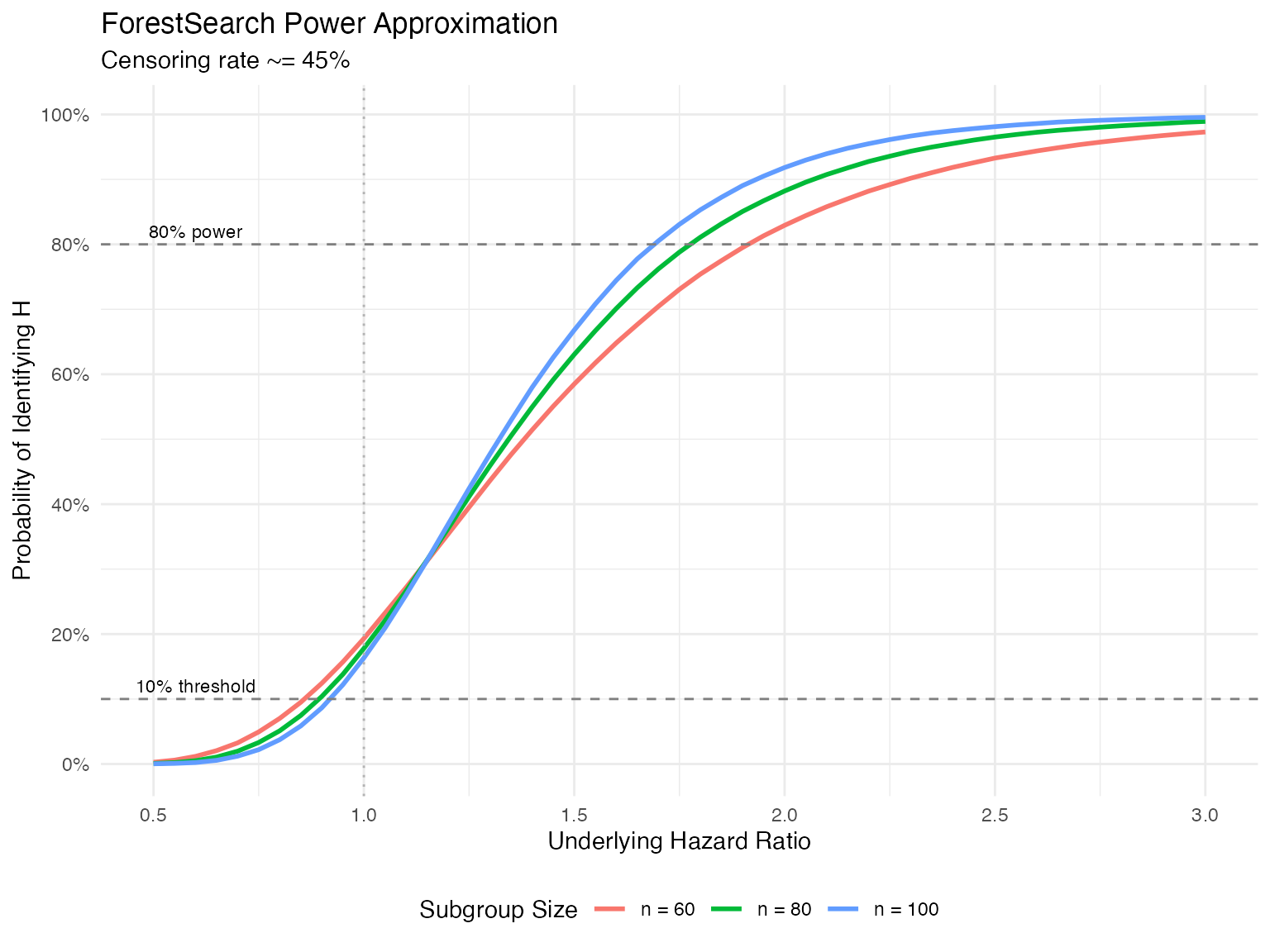
Approximate probability of finding H via ForestSearch

Code

# Power approximation function
approx_power <- function(hr, n_subgroup, cens_rate = 0.45) {
  beta <- log(hr)
  d <- (1 - cens_rate) * n_subgroup
  var_split <- 8 / d

  # Numerical integration
  integrate_2d <- function(beta, var) {
    # Use Monte Carlo integration
    set.seed(123)
    n_sim <- 100000
    w1 <- rnorm(n_sim, mean = beta, sd = sqrt(var))
    w2 <- rnorm(n_sim, mean = beta, sd = sqrt(var))

    mean((w1 + w2 >= 2 * log(1.25)) & (w1 >= 0) & (w2 >= 0))
  }

  integrate_2d(beta, var_split)
}

# Calculate power curves
hr_seq <- seq(0.5, 3.0, by = 0.05)
n_values <- c(60, 80, 100)

power_data <- expand.grid(hr = hr_seq, n = n_values)
power_data$power <- mapply(approx_power, power_data$hr, power_data$n)
power_data$n <- factor(power_data$n, labels = paste("n =", n_values))

library(ggplot2)
ggplot(power_data, aes(x = hr, y = power, color = n)) +
  geom_line(linewidth = 1) +
  geom_hline(yintercept = 0.10, linetype = "dashed", color = "gray50") +
  geom_hline(yintercept = 0.80, linetype = "dashed", color = "gray50") +
  geom_vline(xintercept = 1.0, linetype = "dotted", color = "gray70") +
  scale_x_continuous(breaks = seq(0.5, 3.0, by = 0.5)) +
  scale_y_continuous(breaks = seq(0, 1, by = 0.2), labels = scales::percent) +
  labs(
    x = "Underlying Hazard Ratio",
    y = "Probability of Identifying H",
    color = "Subgroup Size",
    title = "ForestSearch Power Approximation",
    subtitle = "Censoring rate ~= 45%"
  ) +
  theme_minimal() +
  theme(legend.position = "bottom") +
  annotate("text", x = 0.6, y = 0.12, label = "10% threshold", size = 3) +
  annotate("text", x = 0.6, y = 0.82, label = "80% power", size = 3)

Threshold Selection Rationale

The choice of the 1.25 and 1.0 thresholds was based on the desire to control the rate for finding a subgroup $H$ to be approximately 10% when the underlying hazard ratio for $H$ is below 1.0.

If the underlying treatment effect is uniform and beneficial, then for a random subgroup $H$, Cox model estimates will randomly fluctuate around the ITT effect. Because ForestSearch seeks subgroups with evidence for harm (via the screening and consistency thresholds), the chance of forming subgroups under the null with an estimated benefit randomly in favor of control is less likely the stronger the (uniform) ITT treatment effect.

Example: For $\theta^{\dagger}(H) \equiv \theta^{\dagger}(\text{ITT}) = 0.75$, the approximation yields:

Subgroup size	Type-1 error ($\theta^{\dagger}(H) = 0.75$)	$\approx$ 80% power at
$n = 60$	4.9%	HR $\approx$ 1.94
$n = 80$	3.3%	HR $\approx$ 1.81
$n = 100$	2.2%	HR $\approx$ 1.73

Table: Type-1 error and approximate 80% power thresholds.

Bootstrap Bias Correction

Sources of Bias

By the nature of the ForestSearch procedure, we expect unadjusted Cox model estimates based on $\widehat{H}$ to be upwardly biased due to the hazard ratio thresholds (since by construction, point estimates are $\ge 1.25$ for $\widehat{H}$).

However, the bias can also be pressured in the opposite direction depending on:

• The proportion of $H^c$ subjects incorrectly included in $\widehat{H}$
• The value of $\theta^{\dagger}(H)$ relative to $\theta^{\dagger}(H^c)$ (e.g., a mixture of $\theta^{\dagger}(H) = 2.0$ vs. $\theta^{\dagger}(H^c) = 0.65$)

Bias-Corrected Estimator

For bias correction, we proceed on the Cox regression coefficient scale, denoted $\hat{\beta}(\widehat{H})$, and then exponentiate to obtain point estimates and confidence intervals for hazard ratios $\hat{\theta}(\widehat{H}) := \exp(\hat{\beta}(\widehat{H}))$.

Our bias-corrected estimator takes into account two sources of bias involving the discrepancies between the bootstrapped and observed data Cox estimators. The approach is along the lines of Harrell et al. (1996), but additionally incorporates the bias term $\hat{\beta}_b^*(\widehat{H}) - \hat{\beta}(\widehat{H})$.

Notation

For the observed data with estimated subgroup $\widehat{H}$:

• $\hat{\beta}(\widehat{H})$: Estimated Cox model regression parameter

For bootstrap samples $b = 1, \ldots, B$ with estimated subgroup $\widehat{H}^*_b$:

• $\hat{\beta}^*_b(\widehat{H}^*_b)$: Cox model parameter for bootstrap sample based on bootstrap-estimated subgroup
• $\hat{\beta}(\widehat{H}^*_b)$: Cox model parameter for observed data based on bootstrap-estimated subgroup
• $\hat{\beta}^*_b(\widehat{H})$: Cox model parameter for bootstrap sample based on observed subgroup

Bias Terms

Define the bias terms:

$$\eta^*_b(\widehat{H}^*_b) = \hat{\beta}^*_b(\widehat{H}^*_b) - \hat{\beta}(\widehat{H}^*_b)$$

$$\eta^*_b(\widehat{H}) = \hat{\beta}^*_b(\widehat{H}) - \hat{\beta}(\widehat{H})$$

Bias-Corrected Estimators

The bias-corrected estimators are defined as:

$$\hat{\beta}^*(\widehat{H}) = \hat{\beta}(\widehat{H}) - \frac{1}{B}\sum_{b=1}^{B} \left[\eta^*_b(\widehat{H}^*_b) + \eta^*_b(\widehat{H})\right], \qquad \hat{\theta}^*(\widehat{H}) = \exp\!\left(\hat{\beta}^*(\widehat{H})\right)$$

Similarly for the complement:

$$\hat{\beta}^*(\widehat{H}^c) = \hat{\beta}(\widehat{H}^c) - \frac{1}{B}\sum_{b=1}^{B} \left[\eta^*_b(\widehat{H}^{c*}_b) + \eta^*_b(\widehat{H}^c)\right], \qquad \hat{\theta}^*(\widehat{H}^c) = \exp\!\left(\hat{\beta}^*(\widehat{H}^c)\right)$$

The bootstrap resamples are drawn independently with replacement from the observed data $\{O_i := (V_i, \boldsymbol{Z}_i, Y_i, \Delta_i),\; i = 1, \ldots, N\}$. The full ForestSearch algorithm (including LASSO and/or GRF candidate selection) is mimicked in each bootstrap replicate. In general, the variance induced by the (well-defined) candidate selection algorithm is incorporated by mimicking the algorithm in the bootstrap process.

Infinitesimal Jackknife Variance Estimation

To estimate the variance, we apply an infinitesimal jackknife approximation, viewing the bias-corrected estimators as “bagged estimators.”

Let $O^*_b = \{O^*_{b1}, O^*_{b2}, \ldots, O^*_{bN}\}$ denote bootstrap sample $b$. Let $K^*_{bi} = \#\{O^*_{bj} = O_i\}$ denote the number of times observation $O_i$ is drawn for the $b$th bootstrap sample, and let $\bar{K}^*_i = (1/B)\sum_{b=1}^{B} K^*_{bi}$.

The infinitesimal jackknife variance estimate is:

$$\tilde{V} = \sum_{i=1}^{N} \widetilde{\text{cov}}_i^2$$

where:

$$\widetilde{\text{cov}}_i = \frac{1}{B} \sum_{b=1}^{B} (K^*_{bi} - \bar{K}^*_i) \left[\hat{\beta}(\widehat{H}) - \eta^*_b(\widehat{H}^*_b) - \eta^*_b(\widehat{H}) - \hat{\beta}^*(\widehat{H})\right]$$

The bias-corrected variance is:

$$\hat{V} = \tilde{V} - \frac{N}{B} \tilde{\sigma}^2_B$$

where:

$$\tilde{\sigma}^2_B = \frac{1}{B} \sum_{b=1}^{B} \left[\hat{\beta}(\widehat{H}) - \eta^*_b(\widehat{H}^*_b) - \eta^*_b(\widehat{H}) - \hat{\beta}^*(\widehat{H})\right]^2$$

Confidence intervals for hazard ratios are based on standard normal approximations (exponentiated): $\exp\!\left(\hat{\beta}^* \pm 1.96\sqrt{\hat{V}}\right)$.

Bootstrap Bias Correction Workflow

Cross-Validation

Cross-validation is used for evaluating the quality and stability of the selection algorithm. Two forms are implemented.

N-Fold (Leave-One-Out) Cross-Validation

For N-fold CV, we exclude each subject ($i = 1, \ldots, N$) from the analysis and predict their $\widehat{H}$ (or $\widehat{H}^c$) classification based on the remaining $N-1$ subjects.

Let $\hat{\pi}^{-i}(\boldsymbol{Z}_i)$ denote the $i$th subject’s predicted classification based on the FS procedure without the subject in the analysis. Similarly, $\hat{\pi}(\boldsymbol{Z}_i)$ is the FS classification based on the full sample analysis. Form:

$$\widehat{O}_{CV} = \{\hat{O}_i := (V_i, Y_i, \Delta_i, \hat{\pi}(\boldsymbol{Z}_i), \hat{\pi}^{-i}(\boldsymbol{Z}_i)),\; i = 1, \ldots, N\}.$$

Cox model analyses based on $\hat{\pi}(\cdot)$ subgroups correspond to estimates that are unadjusted for the selection algorithm, whereas $\hat{\pi}^{-i}(\cdot)$ represents an out-of-bag (OOB) classification where each subject is not included in the selection algorithm from which they are classified.

Interpretation:

• Correspondence between $\hat{\pi}(\cdot)$ and $\hat{\pi}^{-i}(\cdot)$ subgroup analysis results may be anticipated, especially for large $N$
• If $\hat{\pi}$ and $\hat{\pi}^{-i}$ are identical, there is no diagnostic value; in contrast, substantial lack of correspondence may suggest underlying instability

K-Fold Cross-Validation

In K-fold CV (e.g., 10-fold):

1. Randomly partition the data into K folds
2. For each fold (leaving these subjects out), select $\widehat{H}$ based on the other K-1 folds
3. Predict the classification for the left-out fold

Since this process depends on the random partition, repeat 50–200 times and summarize correspondence measures across the partitions.

CV Metrics

The sensitivity and positive predictive value metrics are modified by replacing $\widehat{H}$ with $\widehat{H}^{-i}$ and the true $H$ with $\widehat{H}$:

$$\text{sensCV}(\widehat{H}) = \frac{\#\{i \in \widehat{H}^{-i} \cap \widehat{H}\}} {\#\{i \in \widehat{H}\}}, \qquad \text{ppvCV}(\widehat{H}) = \frac{\#\{i \in \widehat{H}^{-i} \cap \widehat{H}\}} {\#\{i \in \widehat{H}^{-i}\}}.$$

Cross-Validation Metrics for ForestSearch

Metric	Description	Interpretation
sensCV(Ĥ)	Proportion of full-analysis Ĥ subjects also classified as Ĥ in CV	Higher = more stable Ĥ identification
sensCV(Ĥᶜ)	Proportion of full-analysis Ĥᶜ subjects also classified as Ĥᶜ in CV	Higher = more stable Ĥᶜ identification
ppvCV(Ĥ)	Proportion of CV Ĥ subjects that match full-analysis Ĥ	Higher = CV predictions align with full analysis
ppvCV(Ĥᶜ)	Proportion of CV Ĥᶜ subjects that match full-analysis Ĥᶜ	Higher = CV predictions align with full analysis
Exact Match	Proportion of CV folds reproducing exact subgroup definition	Higher = algorithm consistently identifies same subgroup

Code

cv_metrics <- data.frame(
  Metric = c("sensCV(Ĥ)", "sensCV(Ĥᶜ)", "ppvCV(Ĥ)",
             "ppvCV(Ĥᶜ)", "Exact Match"),
  Description = c(
    "Proportion of full-analysis Ĥ subjects also classified as Ĥ in CV",
    "Proportion of full-analysis Ĥᶜ subjects also classified as Ĥᶜ in CV",
    "Proportion of CV Ĥ subjects that match full-analysis Ĥ",
    "Proportion of CV Ĥᶜ subjects that match full-analysis Ĥᶜ",
    "Proportion of CV folds reproducing exact subgroup definition"
  ),
  Interpretation = c(
    "Higher = more stable Ĥ identification",
    "Higher = more stable Ĥᶜ identification",
    "Higher = CV predictions align with full analysis",
    "Higher = CV predictions align with full analysis",
    "Higher = algorithm consistently identifies same subgroup"
  )
)

knitr::kable(cv_metrics, caption = "Cross-Validation Metrics for ForestSearch")

Simulation Study

Data-Generating Model

The simulation setting is based on the German Breast Cancer Study Group (GBSG) trial covariate structure. A “super-population” of 5,000 subjects was constructed by resampling from the observed GBSG data while retaining covariate structure. Survival outcomes were generated from a Weibull regression model:

$$\log(T) = \mu + \beta_0 V + \beta_1 V Z_1 Z_3 + \boldsymbol{\beta}_2' \boldsymbol{Z}_2 + \tau \epsilon,$$

where $\epsilon$ follows the standard extreme value distribution, $\tau$ is a dispersion parameter, $\boldsymbol{Z}_2 = (Z_1, Z_2, Z_3, Z_4, Z_5)$, and the interaction $V Z_1 Z_3$ defines the true subgroup $H = \{Z_1 = 1\} \cap \{Z_3 = 1\}$. Parameters $\mu$, $\boldsymbol{\beta}_2$, and $\tau$ were based on Weibull model fits to the observed GBSG data; $\beta_0$ and $\beta_1$ were chosen to generate target marginal hazard ratio effects. A covariate-dependent censoring distribution was generated analogously with an overall censoring rate of approximately 46%.

Scenarios

Three models were evaluated across 20,000 simulations:

Simulation model specifications.

Model	Condition	N	p_H (%)	θ†(ITT)	θ†(H)	θ†(Hc)
M1	Null	700	-	0.70	-	-
M1	Alt	700	13%	0.71	2.0	0.65
M2	Null	500	-	0.69	-	-
M2	Alt	500	20%	0.79	2.0	0.69
M3	Null	300	-	0.55	-	-
M3	Alt	300	30%	0.74	2.0	0.56

Code

sim_models <- data.frame(
  Model = c("M1", "M1", "M2", "M2", "M3", "M3"),
  Condition = c("Null", "Alt", "Null", "Alt", "Null", "Alt"),
  N = c(700, 700, 500, 500, 300, 300),
  `p_H` = c("-", "13%", "-", "20%", "-", "30%"),
  `theta_ITT` = c(0.70, 0.71, 0.69, 0.79, 0.55, 0.74),
  `theta_H` = c("-", "2.0", "-", "2.0", "-", "2.0"),
  `theta_Hc` = c("-", "0.65", "-", "0.69", "-", "0.56"),
  check.names = FALSE
)

knitr::kable(
  sim_models,
  col.names = c("Model", "Condition", "N", "p_H (%)",
                "θ†(ITT)", "θ†(H)", "θ†(Hc)"),
  caption = "Simulation model specifications.",
  align = "ccccccc"
)

Each model was evaluated with and without additional random noise factors ($N(0,1)$ variables completely unrelated to the outcome): 3 noise factors for $M_1$, and 5 noise factors for $M_2$ and $M_3$.

Comparator Methods

ForestSearch was compared against:

• GRF / GRF.60: Generalized random forests targeting RMST, with GRF.60 using a truncated horizon $\tau_{60} = 0.6\min(\tau_0, \tau_1)$ for stability. Requires $\ge$ 6-month RMST benefit for control.
• VT(24) / VT(36): Virtual twins targeting survival rate differences at 24 or 36 months. Requires $\delta \ge 0.225$ in favor of control.

All methods were restricted to subgroups with $\ge$ 60 subjects and maximum tree depth of 2. Classification accuracy is measured by sensitivity and positive predictive value:

$$\text{sens}(\widehat{H}) = \frac{\#\{i \in \widehat{H} \cap H\}}{\#\{i \in H\}}, \qquad \text{ppv}(\widehat{H}) = \frac{\#\{i \in \widehat{H} \cap H\}}{\#\{i \in \widehat{H}\}}.$$

Key Results: Subgroup Identification

Subgroup identification results with noise factors. T1E = type-1 error (any(H) under null); Power = any(H) under alternative; sens(H-hat) = sensitivity for H classification under alternative.

Method	T1E	Power	sens(Ĥ)	T1E	Power	sens(Ĥ)
FS_l	2%	71%	64%	3%	89%	77%
FS_lg	11%	83%	74%	14%	96%	81%
GRF	61%	94%	66%	60%	99%	70%
GRF.60	27%	71%	52%	32%	86%	58%
VT(24)	4%	44%	37%	4%	56%	44%
VT(36)	6%	42%	34%	6%	53%	40%

Code

results <- data.frame(
  Method = c("FS_l", "FS_lg", "GRF", "GRF.60", "VT(24)", "VT(36)"),
  `T1E_M1` = c("2%", "11%", "61%", "27%", "4%", "6%"),
  `Pow_M1` = c("71%", "83%", "94%", "71%", "44%", "42%"),
  `Sens_M1` = c("64%", "74%", "66%", "52%", "37%", "34%"),
  `T1E_M2` = c("3%", "14%", "60%", "32%", "4%", "6%"),
  `Pow_M2` = c("89%", "96%", "99%", "86%", "56%", "53%"),
  `Sens_M2` = c("77%", "81%", "70%", "58%", "44%", "40%"),
  check.names = FALSE
)

knitr::kable(
  results,
  col.names = c("Method", "T1E", "Power", "sens(Ĥ)",
                "T1E", "Power", "sens(Ĥ)"),
  caption = paste(
    "Subgroup identification results with noise factors.",
    "T1E = type-1 error (any(H) under null); Power = any(H) under",
    "alternative; sens(H-hat) = sensitivity for H classification",
    "under alternative."
  ),
  align = "lcccccc"
)

Summary of identification results:

• $FS_l$ maintained type-1 error $\le 3\%$ across all scenarios, including with noise factors, and was the most stable approach
• $FS_{lg}$ had slightly elevated type-1 error (up to 14% with noise, inherited from GRF) but achieved the highest classification accuracy among approaches with well-controlled type-1 error
• GRF had substantially inflated type-1 error (up to 61% with noise) under $M_1$ and $M_2$; intuitively, with the addition of noise factors there was more opportunity to randomly form erroneous splits
• Under $M_3$ (strongest ITT effect, $\theta^{\dagger}(\text{ITT}) = 0.55$), all approaches had better-controlled type-1 error since the chance of forming subgroups with estimates in favor of control is less likely with a more pronounced ITT treatment effect
• The power approximation from (eq-power?) was reasonably accurate across all models

Key Results: Estimation Properties

Estimation properties for $FS_{lg}$ with $B = 300$ bootstrap replicates (based on 1,000 simulations per model with noise factors):

Estimation properties for FS_lg across models M1-M3. Relative bias ranges shown across the three models. Oracle coverage = CI coverage for the oracle (true subgroup) estimate.

Estimator	Rel. bias (marginal)	Rel. bias (CDE)	Oracle coverage
θ̂(Ĥ) observed	9% to 24%	9% to 14%	>= 98%
θ̂*(Ĥ) bias-corrected	-10% to -2.4%	-11.6% to -6.3%	>= 95%
θ̂(Ĥᶜ) observed	0.5% to 5.1%	-9.7% to 2.8%	>= 99%
θ̂*(Ĥᶜ) bias-corrected	2.3% to 10.9%	-4.8% to 4.6%	>= 100%

Code

est_results <- data.frame(
  Estimator = c(
    "θ̂(Ĥ) observed",
    "θ̂*(Ĥ) bias-corrected",
    "θ̂(Ĥᶜ) observed",
    "θ̂*(Ĥᶜ) bias-corrected"
  ),
  `Bias_dagger` = c("9% to 24%", "-10% to -2.4%",
                     "0.5% to 5.1%", "2.3% to 10.9%"),
  `Bias_ddagger` = c("9% to 14%", "-11.6% to -6.3%",
                      "-9.7% to 2.8%", "-4.8% to 4.6%"),
  `Coverage_oracle` = c(">= 98%", ">= 95%", ">= 99%", ">= 100%"),
  check.names = FALSE
)

knitr::kable(
  est_results,
  col.names = c("Estimator", "Rel. bias (marginal)",
                "Rel. bias (CDE)", "Oracle coverage"),
  caption = paste(
    "Estimation properties for FS_lg across models M1-M3.",
    "Relative bias ranges shown across the three models.",
    "Oracle coverage = CI coverage for the oracle (true subgroup) estimate."
  ),
  align = "lccc"
)

The bias-corrected estimators tend to be conservative: underestimating both $\theta^{\dagger}(H)$ and $\theta^{\ddagger}(\widehat{H})$ (“conservative for harm”) while overestimating both $\theta^{\dagger}(H^c)$ and $\theta^{\ddagger}(\widehat{H}^c)$ (“conservative for benefit”). Coverage rates for $\hat{\theta}^*(\widehat{H}^c)$ were $\ge 93\%$ for each target, and the oracle coverage rates for both estimators were $\ge 95\%$.

Applications

GBSG Breast Cancer Trial

The German Breast Cancer Study Group trial ($N = 686$) compared tamoxifen (hormonal therapy) to chemotherapy for tumor recurrence. The observed censoring rate was approximately 56%, and the Cox ITT hazard ratio estimate was 0.69 (95% CI: 0.54, 0.89). Seven baseline prognostic factors were available.

ForestSearch results: Using the selection criterion for the largest subgroup with consistency $\ge$ 90%, with LASSO followed by quartile cuts on continuous factors, and GRF ($GRF_{60}$) for additional candidate selection:

• $\widehat{H}$ = Estrogen = 0 (consistency rate 95.1%)
• $\hat{\theta}^*(\widehat{H}) = 1.58$ (0.86, 2.9) — 82 subjects (12%)
• $\hat{\theta}^*(\widehat{H}^c) = 0.64$ (0.44, 0.93) — 604 subjects (88%)

The bias-corrected estimate for $H^c$ suggests a slightly stronger benefit (0.64 vs 0.69 for ITT) that is statistically significant.

Cross-validation: N-fold CV showed perfect stability (all 686 training sets reproduced Estrogen = 0). Across 200 random 10-fold CV analyses, the median number of folds identifying a subgroup was 9/10, with $\text{sensCV}(\widehat{H}) = 73\%$ and $\text{ppvCV}(\widehat{H}) = 83\%$.

Biological plausibility: Tamoxifen is a selective estrogen receptor (ER) modulator with limited efficacy in ER-negative tumors. A patient-level meta-analysis by the Early Breast Cancer Trialists’ Collaborative Group found for ER-negative (ER = 0) subjects, the event-rate ratio was 1.11 (SE = 0.13); whereas for ER-positive ($\ge 10\%$) subjects it was 0.62 (SE = 0.03).

ACTG-175 HIV Trial

The ACTG-175 study ($N = 1{,}083$) compared zidovudine + didanosine (experimental) to didanosine monotherapy (control). The survival outcome was the first occurrence of CD4 decline $\ge$ 50, AIDS progression, or death. The Cox ITT hazard ratio estimate was 0.84 (0.65, 1.09), with 15 baseline covariates available.

Goal: Identify a subgroup with substantial benefit by reversing treatment roles (screening threshold $\log(1/0.6)$, consistency threshold $\log(1/0.8)$), selecting the largest subgroup with consistency $\ge$ 90%.

ForestSearch results:

• $\widehat{Q}$ = Preanti $\le$ 744.5 and Age $>$ 34 (consistency 92.8%)
• $\hat{\theta}^*(\widehat{Q}) = 0.59$ (0.37, 0.94) — 382 subjects (35%)
• $\hat{\theta}^*(\widehat{Q}^c) = 0.95$ (0.65, 1.41) — 701 subjects (65%)

The bias-corrected estimate suggests a relatively strong benefit (0.59 vs 0.84 for ITT) that is statistically significant.

Cross-validation: N-fold CV reproduced the full analysis subgroup definition in all but 7 of 1,083 training sets. The N-fold predicted Cox estimate was 0.59 (0.37, 0.94), identical to the bootstrap bias-corrected estimate. Across 200 random 10-fold analyses, median 9/10 folds identified a subgroup with $\text{sensCV}(\widehat{Q}) \approx 69\%$.

Biological plausibility: The finding aligns with the HIV Trialists’ Collaborative Group meta-analysis reporting greater treatment effects among participants with no previous antiretroviral therapy or higher baseline CD4 counts. Of the $\widehat{Q}$ subgroup, 46.9% were antiretroviral treatment naive.

Variable Selection Methods

LASSO

LASSO (Least Absolute Shrinkage and Selection Operator) is used for Cox model covariate (prognostic) selection via glmnet. In simulations, LASSO helps mitigate false discovery when analyses include baseline factors that are completely random noise.

# LASSO is enabled by default
result <- forestsearch(
  df.analysis = data,
  use_lasso = TRUE,
  use_grf = FALSE,
  ...
)

Generalized Random Forests (GRF)

GRF targets RMST (Restricted Mean Survival Time) via causal survival forests and can be used as a complementary variable selection method. In ForestSearch, GRF is used for identifying candidate factors (binary splits) rather than as the primary identification procedure.

# Enable both LASSO and GRF
result <- forestsearch(
  df.analysis = data,
  use_lasso = TRUE,
  use_grf = TRUE,
  ...
)

Recommendations

Scenario	Recommendation
Standard analysis	use_lasso = TRUE, use_grf = FALSE
Exploratory with many candidates	use_lasso = TRUE, use_grf = TRUE
When noise factors may be present	Always include LASSO
Large datasets with complex interactions	Consider GRF for variable importance

Table: Variable selection recommendations.

In the ACTG-175 analysis, when 20 random noise factors were artificially added without LASSO, ForestSearch identified a nonsensical subgroup based on a noise factor. In contrast, when LASSO was included, the same subgroup and essentially the same bootstrap bias-corrected estimates were obtained.

Practical Considerations

Sample Size Requirements

• Minimum subgroup size: 60 subjects (default n.min = 60)
• Minimum events: 10–12 per treatment arm (default d0.min = 12, d1.min = 12)
• Recommended trial size: $N \ge 300$ for Phase 2; $N \ge 500$ for Phase 3

Computational Considerations

The computational time depends on the number of candidate factors ($K$), the number of subgroup combinations meeting size criteria ($S$), the number of consistency splits (fs.splits, default 400–1000), the number of bootstrap iterations ($B$, typically 300–2000), and the number of CV repetitions.

Typical timing (Apple M1, 20 cores):

Component	Time
FS analysis	$\sim$ 0.05–0.2 minutes
2000 bootstraps	$\sim$ 29–30 minutes
N-fold CV	$\sim$ 4–22 minutes
200 $\times$ 10-fold CV	$\sim$ 59–105 minutes

Table: Computational timing for ForestSearch. Parallel computing is implemented via the doFuture package.

Interpretation Guidelines

1. Bias-corrected estimates should be reported alongside unadjusted estimates
2. Cross-validation metrics provide diagnostic value for stability
3. Biological plausibility should be evaluated using external knowledge (e.g., patient-level meta-analyses of randomized trials)
4. Results are exploratory and should inform future trial design rather than definitive conclusions
5. Conservative estimation: the bias-corrected estimators tend to underestimate harm and overestimate benefit, which is a favorable property for exploratory subgroup analyses
6. Caution against extrapolation: findings should not be extrapolated to comparisons of regimens other than the control regimens studied

References

Athey, Susan, Julie Tibshirani, and Stefan Wager. 2019. “Generalized Random Forests.” The Annals of Statistics 47 (2): 1148–78.

Session Information

sessionInfo()

## R version 4.5.1 (2025-06-13)
## Platform: aarch64-apple-darwin20
## Running under: macOS Tahoe 26.3
## 
## Matrix products: default
## BLAS:   /Library/Frameworks/R.framework/Versions/4.5-arm64/Resources/lib/libRblas.0.dylib 
## LAPACK: /Library/Frameworks/R.framework/Versions/4.5-arm64/Resources/lib/libRlapack.dylib;  LAPACK version 3.12.1
## 
## locale:
## [1] en_US.UTF-8/en_US.UTF-8/en_US.UTF-8/C/en_US.UTF-8/en_US.UTF-8
## 
## time zone: America/Los_Angeles
## tzcode source: internal
## 
## attached base packages:
## [1] stats     graphics  grDevices utils     datasets  methods   base     
## 
## other attached packages:
## [1] ggplot2_4.0.2     DiagrammeR_1.0.11
## 
## loaded via a namespace (and not attached):
##  [1] gtable_0.3.6       jsonlite_2.0.0     dplyr_1.2.0        compiler_4.5.1    
##  [5] tidyselect_1.2.1   jquerylib_0.1.4    systemfonts_1.3.1  scales_1.4.0      
##  [9] textshaping_1.0.4  yaml_2.3.12        fastmap_1.2.0      R6_2.6.1          
## [13] generics_0.1.4     knitr_1.51         htmlwidgets_1.6.4  visNetwork_2.1.4  
## [17] tibble_3.3.1       desc_1.4.3         bslib_0.10.0       pillar_1.11.1     
## [21] RColorBrewer_1.1-3 rlang_1.1.7        cachem_1.1.0       xfun_0.56         
## [25] fs_1.6.6           sass_0.4.10        S7_0.2.1           otel_0.2.0        
## [29] cli_3.6.5          withr_3.0.2        pkgdown_2.2.0      magrittr_2.0.4    
## [33] digest_0.6.39      grid_4.5.1         rstudioapi_0.18.0  lifecycle_1.0.5   
## [37] vctrs_0.7.1        evaluate_1.0.5     glue_1.8.0         farver_2.1.2      
## [41] ragg_1.5.0         rmarkdown_2.30     tools_4.5.1        pkgconfig_2.0.3   
## [45] htmltools_0.5.9