Fit Cox Model with Cubic Spline for Treatment Effect Heterogeneity
Source:R/cox_spline_fit.R
cox_cs_fit.RdEstimates treatment effects as a function of a continuous covariate using a Cox proportional hazards model with natural cubic splines. The function models treatment-by-covariate interactions to detect effect modification.
Usage
cox_cs_fit(
  df,
  tte_name = "os_time",
  event_name = "os_event",
  treat_name = "treat",
  strata_name = NULL,
  z_name = "bm",
  alpha = 0.2,
  spline_df = 3,
  z_max = Inf,
  z_by = 1,
  z_window = 0,
  z_quantile = 0.9,
  show_plot = TRUE,
  plot_params = NULL,
  truebeta_name = NULL,
  verbose = TRUE
)
Arguments
- df
Data frame containing survival data
- tte_name
Character string specifying time-to-event variable name. Default: "os_time"
- event_name
Character string specifying event indicator variable name (1=event, 0=censored). Default: "os_event"
- treat_name
Character string specifying treatment variable name (1=treated, 0=control). Default: "treat"
- strata_name
Character string specifying stratification variable name. If NULL, no stratification is used. Default: NULL
- z_name
Character string specifying continuous covariate name for effect modification. Default: "bm"
- alpha
Numeric value for confidence level (two-sided). Default: 0.20 (80% confidence intervals)
- spline_df
Integer specifying degrees of freedom for natural spline. Default: 3
- z_max
Numeric maximum value for z in predictions. Values beyond this are truncated. Default: Inf (no truncation)
- z_by
Numeric increment for z values in prediction grid. Default: 1
- z_window
Numeric half-width for counting observations near each z value. Default: 0.0 (exact matches only)
- z_quantile
Numeric quantile (0-1) for upper limit of z profile. Default: 0.90 (90th percentile)
- show_plot
Logical indicating whether to display plot. Default: TRUE
- plot_params
List of plotting parameters (see Details). Default: NULL
- truebeta_name
Character string specifying variable containing true log(HR) values for validation/simulation. Default: NULL
- verbose
Logical indicating whether to print diagnostic information. Default: TRUE
Value
List containing:
- z_profile
Vector of z values where treatment effect is estimated
- loghr_est
Point estimates of log(HR) at each z value
- loghr_lower
Lower confidence bound
- loghr_upper
Upper confidence bound
- se_loghr
Standard errors of log(HR) estimates
- counts_profile
Number of observations near each z value
- cox_primary
Log(HR) from standard Cox model (no interaction)
- model_fit
The fitted coxph model object
- spline_basis
The natural spline basis object
Details
Model Structure
The function fits: $$h(t|Z,A) = h_0(t) \exp(\beta_0 A + f(Z) + g(Z) \cdot A)$$
Where:
A is treatment (0/1)
Z is the continuous effect modifier
f(Z) is modeled with natural splines (main effect)
g(Z) is modeled with natural splines (interaction)
The log hazard ratio is: \(\beta(Z) = \beta_0 + g(Z)\)
Plot Parameters
The plot_params argument accepts a list with:
xlab: x-axis labelmain_title: plot titleylimit: y-axis limits c(min, max)y_pad_zero: padding below zero liney_delta: extra space for count labelscex_legend: legend text sizecex_count: count text sizeshow_cox_primary: show standard Cox estimate lineshow_null: show null effect line (log(HR)=0)show_target: show target effect line (e.g., log(0.80))
Examples
# \donttest{
# Simulate data
set.seed(123)
df <- data.frame(
os_time = rexp(500, 0.01),
os_event = rbinom(500, 1, 0.7),
treat = rbinom(500, 1, 0.5),
bm = rnorm(500, 50, 10)
)
# Fit model
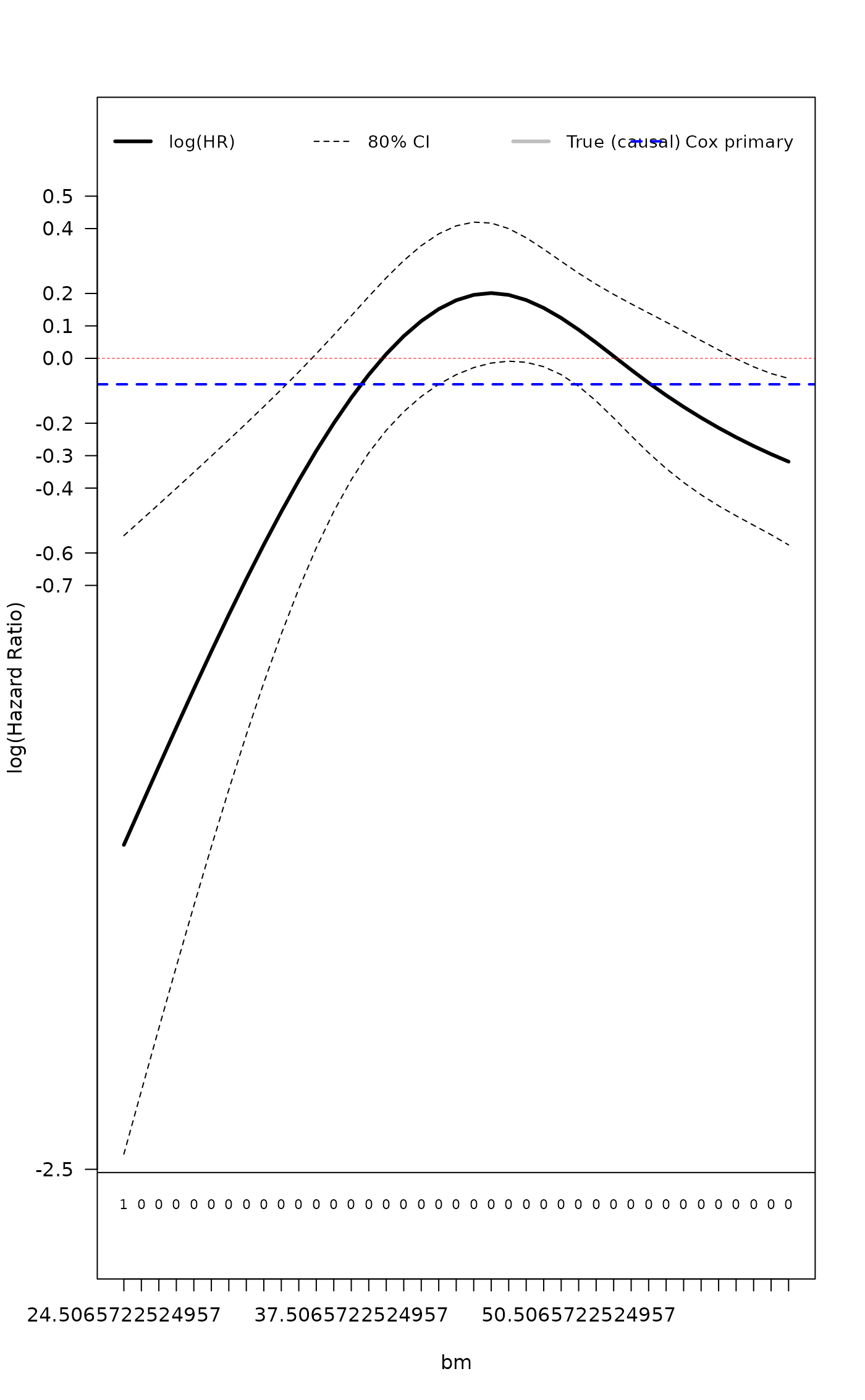
result <- cox_cs_fit(df, z_name = "bm", alpha = 0.20)
#>
#> === Z Variable Summary ===
#> Range: 24.51 83.9
#> Quantiles (75%, 80%, 90%): 56.23 57.9 62.96
#> Prediction grid: 39 points from 24.51 to 62.51
#>
#> === Primary Cox Model ===
#> Treatment log(HR): -0.08
#> Treatment HR: 0.923
#>
#> === Spline Model ===
#> Number of parameters: 7
#> Treatment main effect: -1.5
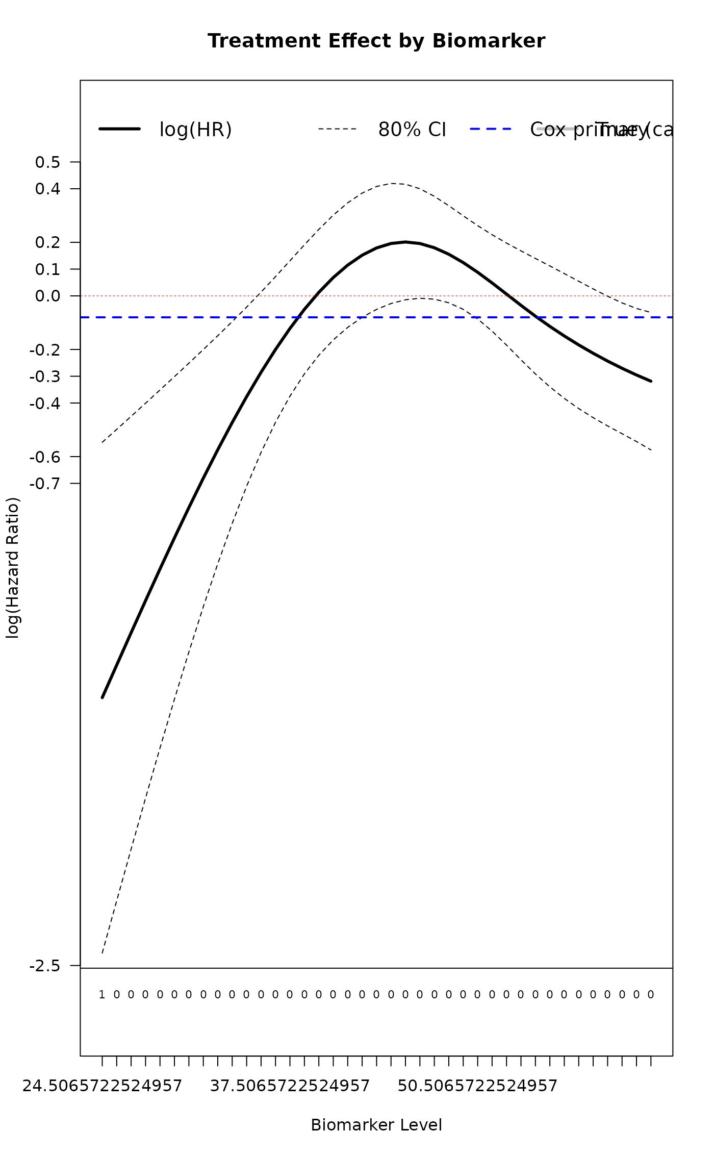
 # Custom plotting
result <- cox_cs_fit(
df,
z_name = "bm",
plot_params = list(
xlab = "Biomarker Level",
main_title = "Treatment Effect by Biomarker",
cex_legend = 1.2
)
)
#>
#> === Z Variable Summary ===
#> Range: 24.51 83.9
#> Quantiles (75%, 80%, 90%): 56.23 57.9 62.96
#> Prediction grid: 39 points from 24.51 to 62.51
#>
#> === Primary Cox Model ===
#> Treatment log(HR): -0.08
#> Treatment HR: 0.923
#>
#> === Spline Model ===
#> Number of parameters: 7
#> Treatment main effect: -1.5
# Custom plotting
result <- cox_cs_fit(
df,
z_name = "bm",
plot_params = list(
xlab = "Biomarker Level",
main_title = "Treatment Effect by Biomarker",
cex_legend = 1.2
)
)
#>
#> === Z Variable Summary ===
#> Range: 24.51 83.9
#> Quantiles (75%, 80%, 90%): 56.23 57.9 62.96
#> Prediction grid: 39 points from 24.51 to 62.51
#>
#> === Primary Cox Model ===
#> Treatment log(HR): -0.08
#> Treatment HR: 0.923
#>
#> === Spline Model ===
#> Number of parameters: 7
#> Treatment main effect: -1.5
 # }
# }