This article is the simulation side of the regional-consistency strategy: how the report’s data-generating mechanism and cells were built, the analytic layer that predicts the design’s behaviour before any simulation, the committed campaign’s results, and how the case study of the application article (mrct-consistency) was found. It executes independently of that article: the case study’s objects, which the checks below compare against, are recomputed first (Section 1).
How replicate 5 was generated: the report’s simulation design
Replicate 5 is one trial drawn from the report’s S2 cell. This section is that design: the data-generating mechanism built from ACTG 175 (Section 3.1), the eight cells, the analytic layer (Section 3.3), and the rule and the calls by which replicate 5 was found and redrawn (Section 3.4); it closes with what can be said about replicate 5 only because it is simulated (Section 3.5).
The data-generating mechanism, built from ACTG 175
A Weibull accelerated-failure-time model is fitted to a published trial and expanded to a super-population of 20,000 rows by a Gaussian copula. A region of about 20% of patients is planted by a logistic model with odds ratio 3 on symptomatic status and no CD4 term, and its baseline hazard is shifted by ; every patient’s hazard ratio is outside = {CD4 230} and inside it, in every region; all hazards are then multiplied by . Three calls build it, shown here as a reader would make them with their own trial.
1. The trial data. ACTG 175 (speff2trial), arms ZDV + ddI (arms == 1, experimental) and ddI alone (arms == 3, control). The outcome is days to the composite endpoint, in months, with event indicator cens; the prognostic covariates are age, weight (wtkg), Karnofsky score (karnof), days of prior antiretroviral therapy (preanti), baseline CD4 (cd40) and CD8 (cd80) counts, and the binary haemophilia (hemo), homosexual activity (homo), drug use (drugs), race, gender and symptomatic status (symptom).
Code
actg <- subset(speff2trial::ACTG175, arms %in% c(1L, 3L))
actg$treat_mrct <- as.integer(actg$arms == 1L)   # ZDV + ddI = 1, ddI = 0
actg$time_months <- actg$days / 30.4375
rownames(actg) <- NULL
c(patients = nrow(actg), events = sum(actg$cens), experimental = sum(actg$treat_mrct))
    patients       events experimental
        1083          231          522
2. The region and the harmed subgroup. inject_mrct_structure() fits the Weibull model on the twelve covariates, expands it by the copula, plants the region (region: prevalence, the logistic model’s odds ratios, the prognostic log hazard ratio ) and the harmed subgroup (spline_spec sets everywhere; x3 multiplies it by in CD4 230), here for cell S2 (). The copula’s latent correlation is fitted live by latentcor (Suggests); without latentcor the call warns and uses the normal-score correlation instead, which gives a valid but different super-population.
Code
dgm_live <- inject_mrct_structure(
  actg,
  outcome_var = "time_months", event_var = "cens", treatment_var = "treat_mrct",
  continuous_vars = c("age", "wtkg", "karnof", "preanti", "cd40", "cd80"),
  factor_vars = c("hemo", "homo", "drugs", "race", "gender", "symptom"),
  x_pred = "cd40",
  spline_spec = list(knot = 300, zeta = 800, log_hrs = rep(log(0.55), 3)),  # b = 0.55
  region = list(prevalence = 0.20, or_pred = 1, x1_vars = "symptom", or_x1 = 3,
                loghr = -log(4),                                          # r
                band = list(cut = 230, or = 1)),
  x3 = list(vars = "cd40", cuts = list(cd40 = 230), loghr = log(2 / 0.55)),  # h = 2 in H*
  region_treat_loghr = NULL,
  n_super = 20000, expand = "copula", seed = 7L,
  continuous_vars_cens = c("age", "cd40"), factor_vars_cens = "symptom")
3. The hazard scale. scale_dgm_hazard() multiplies every hazard by on both arms, by shifting the fitted Weibull intercept (Section 5, the DGM in closed form), and leaves every hazard ratio unchanged. The Weibull fit to ACTG 175 carries that trial’s own event rate; raises it toward a modern trial’s (the application article gives both rates). The windowed Cox limits move with although no hazard ratio does; the application article’s appendix shows why.
Code
dgm_live <- scale_dgm_hazard(dgm_live, m = 3)
c(rows = nrow(dgm_live$df_super), region = mean(dgm_live$df_super$z_region),
  Hstar = mean(dgm_live$df_super$flag_harm))
     rows    region     Hstar
2.000e+04 2.006e-01 1.569e-01
To use your own trial, change these and nothing else:
- the data frame and its outcome, event and treatment names (
outcome_var, event_var, treatment_var; treatment coded 1 = experimental);
- the covariates (
continuous_vars, factor_vars, binary factors coded 0/1, and the censoring model’s continuous_vars_cens, factor_vars_cens);
- the region model (
region: its prevalence, the covariates that predict membership and their odds ratios, its prognostic log hazard ratio );
-
and its effects: the covariate and cut that define it (
x3, region$band), outside it (spline_spec$log_hrs) and inside it (x3$loghr );
- the analysis window and entry: the analysis time and the uniform entry period used below (
analysis_time = 40, max_entry = 11), and cens_adjust for the dropout model.
Reproducing this report’s build exactly
This chunk exists only so that the committed record is reproduced to the last digit on any platform: it builds the cells with the latent correlation stored with the campaign’s build (latent_R.csv, passed as latent_R), so no latentcor fit is made. A reader never needs it. Everything from the build check onward uses the cells built here (build_cell()).
Code
latent_R <- as.matrix(mrct_record("latent_R.csv", row.names = 1))

# One cell: hazard ratio h in H* = {CD4 <= 230}, b = 0.55 elsewhere, region
# prognostic log-HR r, all hazards x m; the calls of steps 2 and 3 above.
build_cell <- function(h, r = -log(4), b = 0.55, cut = 230, m = 3) {
  mrct_build_dgm(
    actg,
    outcome_var = "time_months", event_var = "cens", treatment_var = "treat_mrct",
    continuous_vars = c("age", "wtkg", "karnof", "preanti", "cd40", "cd80"),
    factor_vars = c("hemo", "homo", "drugs", "race", "gender", "symptom"),
    x_pred = "cd40",
    spline_spec = list(knot = 300, zeta = 800, log_hrs = rep(log(b), 3)),
    region = list(prevalence = 0.20, or_pred = 1, x1_vars = "symptom", or_x1 = 3,
                  loghr = r, band = list(cut = cut, or = 1)),
    x3 = list(vars = "cd40", cuts = list(cd40 = cut), loghr = log(h / b)),
    region_treat_loghr = NULL,
    n_super = 20000, expand = "copula", seed = 7L,
    continuous_vars_cens = c("age", "cd40"), factor_vars_cens = "symptom",
    latent_R = latent_R,
    m = m)
}
t_build <- proc.time()[["elapsed"]]
dgm_S2 <- build_cell(h = 2)
t_build <- proc.time()[["elapsed"]] - t_build
# the live fit of step 2 against the shipped matrix
R_live <- dgm_live$mrct$latent_R
R_diff <- if (is.null(R_live)) NA_real_ else max(abs(R_live[rownames(latent_R), colnames(latent_R)] - latent_R))
live_same <- isTRUE(R_diff == 0) && identical(dgm_live$df_super, dgm_S2$df_super)
c(seconds = round(t_build, 1), rows = nrow(dgm_S2$df_super), latent_R_max_abs_diff = R_diff,
  super_population_identical = live_same)
                   seconds                       rows
              5.000000e-01               2.000000e+04
     latent_R_max_abs_diff super_population_identical
              2.858824e-15               0.000000e+00
On this render machine the live fit of step 2 differs from the shipped matrix (largest absolute difference 2.9e-15), so the reader’s path gives a slightly different super-population; the checks below use this chunk’s build.
Build check. The build must equal the campaign’s build record of S2 (build_full_summary.csv, the S2_rmlog4 row) in every numeric column that describes the build; the article stops otherwise.
Code
pop_S2 <- ahr_population(dgm_S2, analysis_time = 40, max_entry = 11)
e_reg <- ahr_limit(pop_S2, "region", b = 0.55, h = 2, variance = FALSE)
e_non <- ahr_limit(pop_S2, "nonregion", b = 0.55, h = 2, variance = FALSE)
ds <- dgm_S2$df_super; reg_s <- ds$z_region == 1; Hs_s <- ds$flag_harm == 1; rg <- dgm_S2$mrct$region
ours <- c(
  h = 2, r = -log(4), mu = unname(dgm_S2$model_params$mu), mu_fitted = unname(dgm_S2$mrct$mu_fitted),
  tau = dgm_S2$model_params$tau, m = dgm_S2$mrct$hazard_multiplier,
  b0_z_region = unname(dgm_S2$model_params$b0["z_region"]), b0_treat = unname(dgm_S2$model_params$b0["treat"]),
  b0_treat_harm = unname(dgm_S2$model_params$b0["treat_harm"]),
  prognostic_loghr_recorded = rg$prognostic_loghr, region_alpha0 = rg$alpha0,
  region_coef_cd40 = unname(rg$coefs["cd40"]), region_coef_symptom = unname(rg$coefs["symptom"]),
  region_coef_cd4_le_230 = log(rg$band$or), prevalence = mean(reg_s),
  Hstar_share_region = mean(Hs_s[reg_s]), Hstar_share_nonregion = mean(Hs_s[!reg_s]),
  event_prob_40_region = e_reg$d, event_prob_40_nonregion = e_non$d,
  events_n1000_region = 1000 * mean(reg_s) * e_reg$d, events_n1000_nonregion = 1000 * mean(!reg_s) * e_non$d,
  mean_theta0_region = mean(ds$theta_0[reg_s]), mean_theta0_nonregion = mean(ds$theta_0[!reg_s]),
  n_build_warnings = length(attr(dgm_S2, "build_warnings")))
br <- mrct_record("build_full_summary.csv"); br <- br[br$cell == "S2_rmlog4", ]
num_cols <- names(br)[vapply(br, is.numeric, NA)]
stopifnot(nrow(br) == 1,
          setequal(setdiff(num_cols, names(ours)), c("prevalence_trials", "seed", "truth_seed", "replicates")),
          isTRUE(all.equal(unname(ours), unname(unlist(br[names(ours)])), tolerance = 1e-8)),
          all((ds$z_cd40 <= 230) == (ds$flag_harm == 1)))
build_diff <- max(abs(ours - unlist(br[names(ours)])) / pmax(1, abs(unlist(br[names(ours)]))))
c(columns_compared = length(ours), largest_relative_difference = signif(build_diff, 2))
           columns_compared largest_relative_difference
                    2.4e+01                     3.8e-15
Passed: the build equals the record (largest relative difference 3.8e-15). In this build the region holds 20.1% of the super-population, holds 15.7% of all patients (16.5% of the region and 15.5% outside it), and at equal covariates a region patient has = 0.25 times the hazard of a non-region patient. The trial: , 1:1, entry uniform over 11 months, analysis at 40 months; the Weibull dropout is pushed far beyond the window (cens_adjust = 50), so all censoring is administrative.
The cells
Six cells at differ only in the hazard ratio inside ; two later-enrolling cells keep S2’s effects and let the region enter later, with or the delay solved so that P(trigger) = 0.25 (Section 3.3.1). The specifications as the committed runs’ timing records state them:
Code
tf <- mrct_record("timing_full.csv"); ts1 <- mrct_record("timing_S1.csv"); te <- mrct_record("timing_entry_cells.csv")
cells <- rbind(
  data.frame(cell = sub("_rmlog4$", "", tf$setting), h = tf$h, r = -log(4), delay = 0, n = 1000,
             replicates = tf$replicates, seed = tf$seed),
  data.frame(cell = "S1", h = ts1$h[ts1$setting == "S1_rmlog4"], r = -log(4), delay = 0, n = 1000,
             replicates = ts1$replicates[ts1$setting == "S1_rmlog4"], seed = ts1$seed[ts1$setting == "S1_rmlog4"]),
  data.frame(cell = te$setting, h = te$h, r = te$r, delay = te$a, n = te$n, replicates = te$replicates,
             seed = te$seed))
cells <- cells[match(c("N0", "N1", "S1", "S2", "S3", "S4", "S2_D1", "S2_D2"), cells$cell), ]
rownames(cells) <- NULL
# the shipped build record's h and r for the five full cells
bfull <- mrct_record("build_full_summary.csv")
stopifnot(!anyNA(cells$cell), near(bfull$h, cells$h[match(sub("_rmlog4$", "", bfull$cell), cells$cell)]),
          near(bfull$r, -log(4), 1e-12))
find <- ifelse(cells$h == 0.55, "nothing: the same benefit everywhere",
               ifelse(cells$h < 1, "nothing harmful: less benefit in CD4 ≤ 230",
                      ifelse(cells$h == 1, "nothing harmful: no effect in CD4 ≤ 230", "harm in CD4 ≤ 230")))
knitr::kable(data.frame(
  cell = cells$cell, `HR in CD4 ≤ 230; elsewhere` = sprintf("%s; 0.55", formatC(cells$h, format = "fg")),
  `what there is to find` = find,
  `region prognostic shift` = sprintf("r = −log %s", formatC(exp(-cells$r), format = "fg", digits = 4)),
  `region enrols later by` = ifelse(cells$delay == 0, "—", sprintf("%s months", f2(cells$delay))),
  n = big(cells$n), replicates = big(cells$replicates), `call seed` = cells$seed, check.names = FALSE),
  align = "lllllrrr", caption = "The cells. Every patient's hazard ratio is the same in every region.")
The cells. Every patient’s hazard ratio is the same in every region.
| N0 |
0.55; 0.55 |
nothing: the same benefit everywhere |
r = −log 4 |
— |
1,000 |
10,000 |
613600000 |
| N1 |
0.75; 0.55 |
nothing harmful: less benefit in CD4 ≤ 230 |
r = −log 4 |
— |
1,000 |
10,000 |
613700000 |
| S1 |
1; 0.55 |
nothing harmful: no effect in CD4 ≤ 230 |
r = −log 4 |
— |
1,000 |
10,000 |
614600000 |
| S2 |
2; 0.55 |
harm in CD4 ≤ 230 |
r = −log 4 |
— |
1,000 |
10,000 |
613800000 |
| S3 |
3; 0.55 |
harm in CD4 ≤ 230 |
r = −log 4 |
— |
1,000 |
10,000 |
613900000 |
| S4 |
4; 0.55 |
harm in CD4 ≤ 230 |
r = −log 4 |
— |
1,000 |
10,000 |
614000000 |
| S2_D1 |
2; 0.55 |
harm in CD4 ≤ 230 |
r = −log 2 |
11.62 months |
1,000 |
10,000 |
615000000 |
| S2_D2 |
2; 0.55 |
harm in CD4 ≤ 230 |
r = −log 2.946 |
6.00 months |
1,000 |
10,000 |
615100000 |
The analytic layer in brief
For any patient set of such a DGM, analysed at a calendar time with uniform staggered entry and administrative censoring only, the analytic layer computes by quadrature (nothing is drawn) the exact limit of the two-sample Cox estimate on the set (the Struthers–Kalbfleisch root, margHR(40): the set’s windowed Cox limit), its information and robust variance, the expected events, the correlation between nested sets’ estimates, the set’s AHR and CDE, and the normal-approximation probability of the trigger at a trial size. ahr_population() reads the DGM; ahr_limit() gives a set’s four truths; ahr_design() gives the trial-level probabilities; ahr_solve() solves P(trigger) = target in one free parameter. ahr_truths_table() and ahr_design_table() tabulate ahr_limit() and ahr_design() over the cells. Section 5 states the formulas.
Code
t_an <- proc.time()[["elapsed"]]
cells6 <- cells[cells$delay == 0, ]
dgms <- lapply(setNames(cells6$h, cells6$cell), function(h) if (h == 2) dgm_S2 else build_cell(h = h))
pops <- lapply(dgms, ahr_population, analysis_time = 40, max_entry = 11)
sets4 <- c(all = "all patients", nonregion = "non-region", region = "region", region_Gstar = "G* (region minus H*)")
h6 <- setNames(cells6$h, cells6$cell)
truths <- ahr_truths_table(pops, sets = names(sets4), b = 0.55, h = h6)
truths$horizon <- NULL; names(truths)[names(truths) == "marghr"] <- "marghr_40"
# against the committed predictions (the analytic records of the campaign)
pred <- rbind(mrct_record("predictions_full.csv"), mrct_record("predictions_S1.csv"))
pv <- function(cell, q, set) { v <- pred$value[pred$cell == cell & pred$quantity == q & pred$set == set]; stopifnot(length(v) == 1); v }
tr_ref <- mapply(function(c, s, q) pv(paste0(c, "_rmlog4"), q, s),
                 rep(truths$cell, 4), rep(truths$set, 4),
                 rep(c("marghr_40", "marghr_inf", "ahr", "cde"), each = nrow(truths)))
stopifnot(near(unlist(truths[c("marghr_40", "marghr_inf", "ahr", "cde")]), tr_ref))
tt <- truths
tt$set <- sets4[tt$set]; tt[3:6] <- lapply(tt[3:6], f3)
reg_S2 <- truths[truths$cell == "S2" & truths$set == "region", ]
stopifnot(reg_S2$marghr_40 < 1, reg_S2$cde > 1)
knitr::kable(setNames(tt, c("cell", "set", "margHR(40)", "margHR(∞)", "AHR", "CDE")), row.names = FALSE,
             align = "llrrrr", caption = "The four truths of four sets in the six cells at r = −log 4 (ahr_truths_table()); equal to the committed predictions to 1e-9.")
The four truths of four sets in the six cells at r = −log 4 (ahr_truths_table()); equal to the committed predictions to 1e-9.
| N0 |
all patients |
0.595 |
0.663 |
0.550 |
0.550 |
| N0 |
non-region |
0.588 |
0.621 |
0.550 |
0.550 |
| N0 |
region |
0.572 |
0.631 |
0.550 |
0.550 |
| N0 |
G* (region minus H*) |
0.560 |
0.617 |
0.550 |
0.550 |
| N1 |
all patients |
0.632 |
0.677 |
0.577 |
0.620 |
| N1 |
non-region |
0.623 |
0.635 |
0.577 |
0.620 |
| N1 |
region |
0.628 |
0.646 |
0.579 |
0.625 |
| N1 |
G* (region minus H*) |
0.560 |
0.617 |
0.550 |
0.550 |
| S1 |
all patients |
0.667 |
0.689 |
0.604 |
0.708 |
| S1 |
non-region |
0.656 |
0.646 |
0.603 |
0.707 |
| S1 |
region |
0.690 |
0.658 |
0.607 |
0.720 |
| S1 |
G* (region minus H*) |
0.560 |
0.617 |
0.550 |
0.550 |
| S2 |
all patients |
0.743 |
0.711 |
0.673 |
1.059 |
| S2 |
non-region |
0.723 |
0.666 |
0.672 |
1.056 |
| S2 |
region |
0.868 |
0.679 |
0.681 |
1.097 |
| S2 |
G* (region minus H*) |
0.560 |
0.617 |
0.550 |
0.550 |
| S3 |
all patients |
0.777 |
0.720 |
0.718 |
1.409 |
| S3 |
non-region |
0.749 |
0.674 |
0.715 |
1.404 |
| S3 |
region |
0.980 |
0.687 |
0.728 |
1.474 |
| S3 |
G* (region minus H*) |
0.560 |
0.617 |
0.550 |
0.550 |
| S4 |
all patients |
0.796 |
0.725 |
0.751 |
1.760 |
| S4 |
non-region |
0.762 |
0.678 |
0.748 |
1.753 |
| S4 |
region |
1.053 |
0.692 |
0.763 |
1.851 |
| S4 |
G* (region minus H*) |
0.560 |
0.617 |
0.550 |
0.550 |
The four truths differ, and the difference is the point. The AHR and the CDE depend on a set only through its shares; the two marginal ratios are bounded in and depend on the window and the prognostic structure. In S2 the region’s margHR(40) is 0.868, below 1, although its CDE is 1.097: the trigger in S2 is a sampling event around a regional limit below 1.
The trigger predictions at , and the oracle joint, P(trigger and region() < 1.0) — in the application article’s named events, non-consistency and oracle consistency:
Code
# ahr_design_table()'s probabilities, under the names of the committed predictions
design_tab <- function(n, ref_cell) {
  d <- ahr_design_table(pops, b = 0.55, h = h6, n = n)
  data.frame(cell = d$cell, n = d$n, p_A = d$p_itt_ub_lt1, p_B = d$p_region_itt_gt1,
             p_A_B = d$p_trigger, p_Cstar = d$p_region_Gstar_lt1,
             p_A_B_Cstar = d$p_trigger_and_Gstar_lt1, ref = ref_cell(d$cell))
}
d1000 <- design_tab(1000, function(k) paste0(k, "_rmlog4"))
for (q in c("p_A", "p_B", "p_A_B", "p_Cstar", "p_A_B_Cstar"))
  stopifnot(all(abs(d1000[[q]] - vapply(d1000$ref, function(cc) pv(cc, q, ""), 0)) < 1e-9))
show_design <- function(d) knitr::kable(data.frame(
  cell = d$cell, `P(ITT ub < 1.0)` = f3(d$p_A), `P(region ITT > 1.0)` = f3(d$p_B), `P(trigger)` = f3(d$p_A_B),
  `P(region(G*) < 1.0)` = f3(d$p_Cstar), `P(oracle joint)` = f3(d$p_A_B_Cstar),
  `P(G* < 1.0 | trigger)` = f3(d$p_A_B_Cstar / d$p_A_B), check.names = FALSE),
  row.names = FALSE, align = "lrrrrrr")
show_design(d1000)
| N0 |
0.999 |
0.055 |
0.054 |
0.913 |
0.017 |
0.310 |
| N1 |
0.994 |
0.086 |
0.084 |
0.913 |
0.036 |
0.436 |
| S1 |
0.978 |
0.131 |
0.123 |
0.913 |
0.068 |
0.555 |
| S2 |
0.844 |
0.326 |
0.241 |
0.913 |
0.187 |
0.777 |
| S3 |
0.718 |
0.473 |
0.289 |
0.913 |
0.245 |
0.848 |
| S4 |
0.635 |
0.568 |
0.305 |
0.913 |
0.268 |
0.879 |
At (predictions only; the campaign is in the report and is not reproduced here):
Code
pred700 <- rbind(mrct_record("predictions_n700.csv"), mrct_record("predictions_S1.csv"))
pv7 <- function(cell, q) { v <- pred700$value[pred700$cell == cell & pred700$quantity == q & pred700$set == ""]; stopifnot(length(v) == 1); v }
d700 <- design_tab(700, function(k) paste0(k, "_rmlog4_n700"))
for (q in c("p_A", "p_B", "p_A_B", "p_Cstar", "p_A_B_Cstar"))
  stopifnot(all(abs(d700[[q]] - vapply(d700$ref, pv7, 0, q = q)) < 1e-9))
show_design(d700)
| N0 |
0.986 |
0.091 |
0.086 |
0.873 |
0.025 |
0.294 |
| N1 |
0.961 |
0.127 |
0.114 |
0.873 |
0.045 |
0.399 |
| S1 |
0.914 |
0.175 |
0.142 |
0.873 |
0.071 |
0.501 |
| S2 |
0.700 |
0.353 |
0.198 |
0.873 |
0.141 |
0.709 |
| S3 |
0.565 |
0.478 |
0.211 |
0.873 |
0.166 |
0.786 |
| S4 |
0.488 |
0.557 |
0.212 |
0.873 |
0.174 |
0.822 |
Code
reg_lt1 <- truths$cell[truths$set == "region" & truths$marghr_40 < 1]
stopifnot(all(d700$p_B[d700$cell %in% reg_lt1] > d1000$p_B[d1000$cell %in% reg_lt1]))
Both tables equal the committed predictions to . In the cells whose regional limit is below 1 (N0, N1, S1, S2, S3), P(region ITT > 1.0) is larger at than at : there the trigger is a small-sample event, made frequent by the region’s few events.
How was chosen, and the later-enrolling regions
The campaign’s regional shift was chosen to make the trigger frequent at the design: with S2’s effects (), solving P(trigger) = 0.25 at is found by ahr_solve(), and the campaign rounded it to . Each evaluation rebuilds the DGM at that .
Code
p_trig_r <- function(r, delay = NULL) {
  d <- build_cell(h = 2, r = r)
  ahr_design(ahr_population(d, 40, 11, entry_delay = delay), b = 0.55, h = 2, n = 1000)$prob[["p_trigger"]]
}
roots <- mrct_record("entry_roots.csv")
rref <- function(tag) { x <- roots[startsWith(roots$row, tag), ]; stopifnot(nrow(x) == 1); x }
sol_r <- ahr_solve(p_trig_r, 0.25, c(-log(5), -log(3.5)), n_scan = 5L, tol = 1e-10)
ref0 <- rref("Reference: a = 0, r solving")
stopifnot(sol_r$n_roots == 1, abs(sol_r$roots - ref0$r) < 1e-6)
c(root_r = sol_r$roots, k_in_minus_log_k = exp(-sol_r$roots), committed_root = ref0$r,
  P_trigger_at_root = sol_r$values)
           root_r  k_in_minus_log_k    committed_root P_trigger_at_root
        -1.441190          4.225721         -1.441190          0.250000
The root is , the committed -1.4412; the campaign used , where P(trigger) is 0.241. The same target defines the two later-enrolling cells, in which the region’s patients enter months after the others (entry_delay): D1 keeps and solves the delay ; D2 fixes months and solves .
Code
dgm_r2 <- build_cell(h = 2, r = -log(2))
p_trig_a <- function(a) ahr_design(ahr_population(dgm_r2, 40, 11, entry_delay = list(var = "z_region", delay = a)),
                                   b = 0.55, h = 2, n = 1000)$prob[["p_trigger"]]
sol_a <- ahr_solve(p_trig_a, 0.25, c(11, 12), scan = c(11, 12), tol = 1e-8)
sol_r6 <- ahr_solve(p_trig_r, 0.25, c(-log(3.5), -log(2.5)), n_scan = 5L, tol = 1e-10,
                    delay = list(var = "z_region", delay = 6))
d1r <- rref("D1:"); d2r <- rref("D2:")
stopifnot(sol_a$n_roots == 1, abs(sol_a$roots - d1r$a) < 1e-6,
          sol_r6$n_roots == 1, abs(sol_r6$roots - d2r$r) < 1e-6)
# the design layer at the two roots, against the committed root records
dD <- lapply(list(S2_D1 = list(r = -log(2), a = sol_a$roots), S2_D2 = list(r = sol_r6$roots, a = 6)), function(x) {
  d <- if (abs(x$r + log(2)) < 1e-12) dgm_r2 else build_cell(h = 2, r = x$r)
  ahr_design(ahr_population(d, 40, 11, entry_delay = list(var = "z_region", delay = x$a)), 0.55, 2, 1000)
})
for (k in names(dD)) {
  x <- if (k == "S2_D1") d1r else d2r; p <- dD[[k]]$prob
  stopifnot(abs(p[["p_itt_ub_lt1"]] - x$p_itt_ub_lt1) < 1e-6, abs(p[["p_region_itt_gt1"]] - x$p_region_itt_gt1) < 1e-6,
            abs(p[["p_trigger_and_Gstar_lt1"]] - x$p_trigger_Gstar_lt1) < 1e-6)
}
knitr::kable(data.frame(
  cell = c("S2_D1", "S2_D2"), `r` = sprintf("−log %s", f3(exp(-c(-log(2), sol_r6$roots)))),
  `region delay a (months)` = f3(c(sol_a$roots, 6)),
  `P(ITT ub < 1.0)` = f3(vapply(dD, function(d) d$prob[["p_itt_ub_lt1"]], 0)),
  `P(region ITT > 1.0)` = f3(vapply(dD, function(d) d$prob[["p_region_itt_gt1"]], 0)),
  `P(trigger)` = f3(vapply(dD, function(d) d$prob[["p_trigger"]], 0)),
  `P(oracle joint)` = f3(vapply(dD, function(d) d$prob[["p_trigger_and_Gstar_lt1"]], 0)),
  `region margHR(40)` = f3(vapply(dD, function(d) d$sets$marghr[d$sets$set == "region"], 0)),
  check.names = FALSE), row.names = FALSE, align = "lrrrrrrr",
  caption = "The later-enrolling cells: roots reproduced with entry_delay (committed roots to 1e-6).")
The later-enrolling cells: roots reproduced with entry_delay (committed roots to 1e-6).
| S2_D1 |
−log 2.000 |
11.619 |
0.862 |
0.323 |
0.250 |
0.193 |
0.866 |
| S2_D2 |
−log 2.946 |
6.000 |
0.855 |
0.329 |
0.250 |
0.193 |
0.869 |
Code
A later-enrolling region is followed for less time, which keeps its 40-month window in the phase where the treated patients are failing: a delay of 11.62 months at , or of 6 months at , does what the shift to does at no delay. The analytic computations of this section took 34 seconds.
Finding a case study
The report’s case example is one trial of the S2 cell, chosen by a stated rule: the first replicate, by index, that reaches the trigger, declares and has region() < 1.0. Four calls find and examine such a trial in any simulation. They are shown on S2 with the campaign’s arguments and call seed at 100 replicates (nsims_demo, set at the top of the file), on workers from parallel::detectCores(); with the campaign’s seed these replicates are the campaign’s first 100. The same run is summarised beside the campaign in Section 4.6.
1. Simulate with the full record. mrct_region_sims(record = "full") keeps, for every trial, the Cox fits of the patient sets (the "estimators" attribute) that the selection reads.
Code
seed_S2 <- cells$seed[cells$cell == "S2"]
confounders <- analysis_covariates(dgm_S2, "observed")
workers_demo <- max(1L, min(parallel::detectCores(), nsims_demo))
t_demo <- proc.time()[["elapsed"]]
demo <- mrct_region_sims(
  dgm_S2, n_sims = nsims_demo, n_sample = 1000, region_var = "z_region",
  sg_focus = "hrMaxSG", maxk = 2,
  hr.threshold = 0.90, hr.consistency = 0.80, pconsistency.threshold = 0.90,
  confounders.name = confounders, conf_force = character(0),
  fs_args = list(conf.cont_jcuts = list(z_cd40 = 10, z_wtkg = 10, z_preanti = 10),
                 effect_neighborhood = 0.20, use_grf = FALSE, use_lasso = FALSE),
  sim_args = list(rand_ratio = 1, draw_treatment = TRUE, max_entry = 11, cens_adjust = 50),
  analysis_time = 40, cens_adjust = 50,
  parallel_args = list(plan = "multisession", workers = workers_demo, show_message = FALSE),
  details = FALSE, verbose_n_sims = 0, seed = seed_S2, record = "full")
t_demo <- proc.time()[["elapsed"]] - t_demo
future::plan(future::sequential)
c(replicates = nsims_demo, workers = workers_demo, seconds = round(t_demo, 1))
replicates    workers    seconds
     100.0        4.0      308.2
2. Select the trial. mrct_select_case() flags every trial for the trigger, a declaration and region() < 1.0, and returns the first meeting all three.
Code
  sim trigger declared region_Ghat_lt1 hr_itt_all    itt_ub hr_itt_region
1   5    TRUE     TRUE            TRUE  0.8084137 0.9828564        1.0364
  hr_region_Ghat hr_region_Gstar                              sg_found
1      0.8436078       0.7359127 {z_cd40 <= 236} & !{z_preanti <= 196}
Code
# the selection returns replicate 5, the report's case example
stopifnot(nrow(case) == 1, case$sim == 5)
est <- as.data.frame(attr(demo, "estimators")); demo <- as.data.frame(demo)[order(demo$sim), ]
stopifnot(nrow(demo) == nsims_demo, identical(demo$sim, seq_len(nsims_demo)))
# the campaign's first replicates, as the shipped record has them
trials5 <- mrct_record("s2_example_trials.csv")
k5 <- intersect(trials5$sim, demo$sim)
stopifnot(near(demo$hr_itt[match(k5, demo$sim)], trials5$hr_itt[match(k5, trials5$sim)], 1e-10),
          near(demo$hr_test[match(k5, demo$sim)], trials5$hr_region[match(k5, trials5$sim)], 1e-10),
          identical(demo$sg_found[match(k5, demo$sim)], trials5$sg_found[match(k5, trials5$sim)]))
3. Redraw it, and check it against Section 1. mrct_case_study() redraws trial k exactly as the simulation drew it (under L’Ecuyer-CMRG, by simulate_from_dgm() with seed equal to the call seed plus , restoring R’s default generator after), runs the identifier on its non-region patients with the simulation’s arguments (the arguments mrct_region_sims() takes directly go into fs_args here) and analyses the four sets. It runs here with mr_inference = FALSE: the MR draws are made once, in Section 1. The redrawn trial must equal the shipped rep5_trial.csv in every shipped column, to floating-point precision (see the note below the check), and its and four sets those of Section 1; the article stops otherwise.
Code
t_cs <- proc.time()[["elapsed"]]
cs <- mrct_case_study(
  dgm_S2, seed = seed_S2, k = case$sim, n = 1000, region_var = "z_region",
  fs_args = list(sg_focus = "hrMaxSG", maxk = 2,
                 hr.threshold = 0.90, hr.consistency = 0.80, pconsistency.threshold = 0.90,
                 confounders.name = confounders, conf_force = character(0),
                 conf.cont_jcuts = list(z_cd40 = 10, z_wtkg = 10, z_preanti = 10),
                 effect_neighborhood = 0.20, use_grf = FALSE, use_lasso = FALSE),
  sim_args = list(rand_ratio = 1, draw_treatment = TRUE, max_entry = 11, cens_adjust = 50),
  analysis_time = 40, cens_adjust = 50,
  mr_inference = FALSE)
t_cs <- proc.time()[["elapsed"]] - t_cs
Code
# the simulation route against the case study of @sec-case-objects
redraw_rel <- max(vapply(names(trial), function(v) {
  a <- as.numeric(cs$trial[[v]]); b <- as.numeric(trial[[v]])
  max(abs(a - b) / pmax(abs(b), .Machine$double.eps))
}, 0))
stopifnot(RNGkind()[1] == "Mersenne-Twister", seed_S2 + case$sim == seed_rep5,
          cs$call_args$sim_args$seed == seed_rep5, identical(confounders, covs),
          nrow(cs$trial) == nrow(trial), all(names(trial) %in% names(cs$trial)),
          all(vapply(names(trial), function(v) isTRUE(all.equal(as.numeric(cs$trial[[v]]), as.numeric(trial[[v]]), tolerance = 1e-12)), NA)),
          identical(cs$Hhat, Hhat_def), identical(cs$in_Hhat, in_Hhat), identical(cs$sets$set, four$set),
          all(cs$sets$n == four$n, cs$sets$events_exp == four$events_exp, cs$sets$events_ctl == four$events_ctl),
          near(c(cs$sets$hr, cs$sets$lo, cs$sets$hi), c(four$hr, four$lo, four$hi), 1e-12))
knitr::kable(data.frame(set = set_label[four$set], `mrct_case_study()` = f3(cs$sets$hr),
                        `the case study` = f3(four$hr), abs_difference = signif(abs(cs$sets$hr - four$hr), 2),
                        check.names = FALSE), row.names = FALSE, align = "lrrr",
             caption = sprintf("The four hazard ratios by the simulation route and by the case study; Ĥ the same (%s).", Hhat_def))
The four hazard ratios by the simulation route and by the case study; Ĥ the same ({z_cd40 <= 236} & !{z_preanti <= 196}).
| All patients, ITT |
0.808 |
0.808 |
0 |
| Region, ITT |
1.036 |
1.036 |
0 |
| Region minus H* (G*) |
0.736 |
0.736 |
0 |
| Region minus Ĥ (Ĝ) |
0.844 |
0.844 |
0 |
Passed: the redrawn trial equals rep5_trial.csv (largest relative difference 5.3e-15), and its and four hazard ratios (largest absolute difference 0) are those of Section 1. The call took 9 seconds.
Platform precision
rep5_trial.csv was written on the Linux machine that ran the campaign. On another platform the redraw is the same trial, but continuous columns can differ in their last digits, because the linear-algebra library and floating-point arithmetic differ. On macOS (arm64, R 4.5.2, Apple’s Accelerate library), two columns differ, y_sim and z_wtkg, by at most 5e-15 relative, and every integer and 0/1 column is identical. The check therefore compares with a relative tolerance of 1e-12, not exactly.
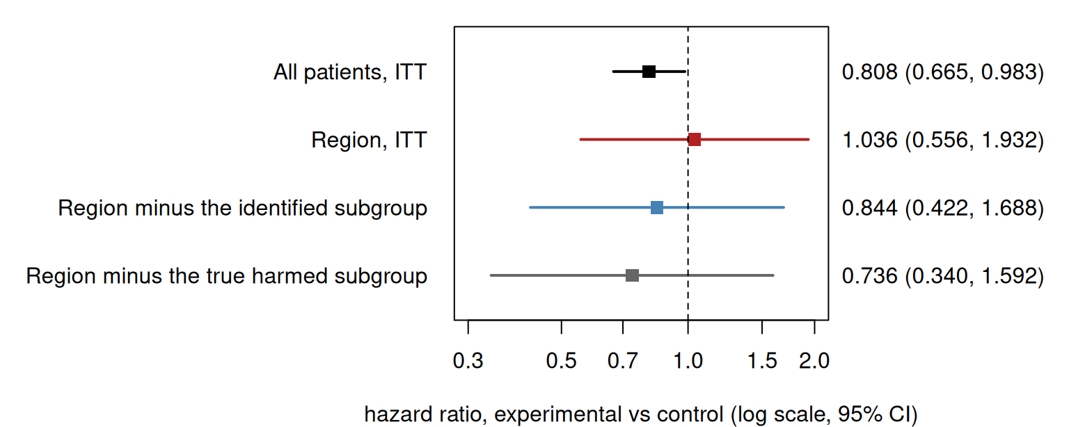
4. Print and plot. The four sets (and, when it is run with mr_inference = TRUE, the multiplier-resampling bounds for and its non-region complement); the forest plot of the four sets (plot(cs) also draws the Kaplan–Meier panels, as in the application article).
Code
MRCT case study: trial 5 (seed 613800000 + 5), n = 1000, region 'z_region'
H-hat: {z_cd40 <= 236} & !{z_preanti <= 196}
Trigger (ITT ub < 1.0 and region ITT > 1.0): TRUE

 Set                        n    exp n/events ctl n/events HR    95% CI
 All patients, ITT          1000 500/187      500/218      0.808 0.665, 0.983
 Region, ITT                 194 104/22       90/18        1.036 0.556, 1.932
 Region minus H* (G*)        159 83/12        76/14        0.736 0.340, 1.592
 Region minus H-hat (G-hat)  174 92/16        82/16        0.844 0.422, 1.688

H-hat against H* (TP, FP, FN, TN):
  nonregion  65, 8, 65, 668
  region     18, 2, 17, 157

Multiplier resampling: not run, or nothing declared.
Code
plot(cs, which = "forest")
The selection returns replicate 5, the report’s case example and the trial of Section 1.
Because this trial is simulated
With a real trial none of this is available: is unknown, so there is no , no oracle and no sensitivity or specificity. This subsection uses the S2 build and the analytic layer, so it is placed here, after them, rather than in the application article.
against , in the region and outside
Code
cc2 <- function(w) c(TP = sum(in_Hhat[w] & Hstar[w]), FP = sum(in_Hhat[w] & !Hstar[w]),
                     FN = sum(!in_Hhat[w] & Hstar[w]), TN = sum(!in_Hhat[w] & !Hstar[w]))
cf_non <- cc2(!reg); cf_reg <- cc2(reg)
stopifnot(identical(cf_non, cs$confusion$nonregion), identical(cf_reg, cs$confusion$region))
sens <- function(x) x[["TP"]] / (x[["TP"]] + x[["FN"]]); spec <- function(x) x[["TN"]] / (x[["TN"]] + x[["FP"]])
knitr::kable(data.frame(population = c("non-region (where the identifier ran)", "region (where Ĥ is applied)"),
                        n = c(sum(!reg), sum(reg)),
                        TP = c(cf_non[["TP"]], cf_reg[["TP"]]), FP = c(cf_non[["FP"]], cf_reg[["FP"]]),
                        FN = c(cf_non[["FN"]], cf_reg[["FN"]]), TN = c(cf_non[["TN"]], cf_reg[["TN"]]),
                        Sens = f3(c(sens(cf_non), sens(cf_reg))), Spec = f3(c(spec(cf_non), spec(cf_reg)))),
             row.names = FALSE, align = "lrrrrrrr",
             caption = "Ĥ against H* = {CD4 ≤ 230}. TP: in Ĥ and in H*; FP: in Ĥ, not in H*; FN: in H*, not in Ĥ.")
Ĥ against H* = {CD4 ≤ 230}. TP: in Ĥ and in H; FP: in Ĥ, not in H; FN: in H*, not in Ĥ.
| non-region (where the identifier ran) |
806 |
65 |
8 |
65 |
668 |
0.500 |
0.988 |
| region (where Ĥ is applied) |
194 |
18 |
2 |
17 |
157 |
0.514 |
0.987 |
Code
hr4 <- setNames(four$hr, four$set)
stopifnot(hr4[["region_Gstar"]] < hr4[["region_Ghat"]], hr4[["region_Ghat"]] < 1, hr4[["itt_region"]] > 1)
has the right variable and nearly the right cut, narrowed by prior therapy: it finds about half of the harmed patients (Sens 0.500 outside the region) and almost no one else (Spec 0.988). Applied in the region it removes 20 patients, 18 of them in , and region() is 0.844, between the whole region and the oracle region() = 0.736, as a partial removal of should.
Reproduction check against the committed record
The four hazard ratios must equal the shipped record to three decimals with the same counts, the committed definition, the tables the committed ones, and the MR values the MR campaign’s record of this replicate (same call, same seed); the article stops otherwise.
Code
rec <- mrct_record("s2_example_four_sets.csv", colClasses = c(hr_3dp = "character", ci_3dp = "character"))
rec <- rec[match(four$set, rec$set), ]
trials5 <- mrct_record("s2_example_trials.csv")
defs <- readLines(system.file("extdata", "mrct-consistency", "s2_example_definitions.md", package = "forestsearch"))
rec2x2 <- function(lab) {
  l <- defs[grepl(paste0("^- ", lab, "( \\(|:)"), defs)]; stopifnot(length(l) == 1)
  vapply(c(TP = "TP", FP = "FP", FN = "FN", TN = "TN"),
         function(k) as.integer(sub(sprintf(".*%s ([0-9]+).*", k), "\\1", l)), 0L)
}
stopifnot(identical(rec$set, four$set), all(rec$sim == 5),
          identical(f3(four$hr), rec$hr_3dp),
          all(four$n == rec$n, four$events_exp == rec$events_exp, four$events_ctl == rec$events_ctl),
          identical(Hhat_def, trials5$sg_found[trials5$sim == 5]),
          identical(cf_reg, rec2x2("Region")), identical(cf_non, rec2x2("Non-region")))
knitr::kable(data.frame(set = set_label[four$set], reproduced = f3(four$hr), committed = rec$hr_3dp,
                        abs_difference = signif(abs(four$hr - rec$hr), 2)), row.names = FALSE,
             caption = "Reproduced against the committed hazard ratios.")
Reproduced against the committed hazard ratios.
| All patients, ITT |
0.808 |
0.808 |
0 |
| Region, ITT |
1.036 |
1.036 |
0 |
| Region minus H* (G*) |
0.736 |
0.736 |
0 |
| Region minus Ĥ (Ĝ) |
0.844 |
0.844 |
0 |
Passed under forestsearch 0.5.0: the four hazard ratios (largest absolute difference 1.6e-15), the counts, and both tables equal the record.
Code
# against the MR campaign's record of this replicate (same call, same seed)
mf <- mrct_record("mr_field_S2_rep5.csv")
stopifnot(nrow(mf) == 1, mf$sim == 5, identical(mf$sg_found, Hhat_def),
          near(c(mv$naive_est[1], mv$debiased_est[1], mv$ij_lower[1], mv$ij_upper[1], mv$field_bound[1],
                 mv$naive_est[2], mv$debiased_est[2], mv$field_bound[2], mv$bonferroni_bound),
               c(mf$naive_H, mf$debiased_H, mf$ij_lower_H, mf$ij_upper_H, mf$field_lower_1s_H,
                 mf$naive_Hc, mf$debiased_Hc, mf$field_upper_1s_Hc, mf$bonf_lower_H, mf$bonf_upper_Hc), 1e-8),
          abs(mr$reselection$p_hat[[mr$selected_index]] - mf$p_hat_H) < 1e-12)
stopifnot(fl$lower_1s < 1, fl$complement$upper_1s < 1, mr$naive$est > mr$debiased$est)
c(p_hat_Hhat = mr$reselection$p_hat[[mr$selected_index]], selection_rate = mr$selection_rate)
    p_hat_Hhat selection_rate
         0.186          1.000
The MR values equal the campaign’s record of this replicate: the naive, de-biased, IJ and field values for and , the Bonferroni pair and the re-selection share.
The four sets beside their limits
The analytic layer’s limit of each set’s Cox estimate, with the set’s AHR and CDE; is replicate 5’s rule applied to every super-population row of the region. is the estimate’s distance from its limit in units of the robust SE that the limit implies at the set’s size.
Code
Hhat_super <- get_dfpred(dgm_S2$df_super, sg.harm = fs$sg.harm, version = 2)$treat.recommend == 0
lim_sets <- list(itt_all = "all", itt_region = "region", region_Gstar = "region_Gstar",
                 region_Ghat = pop_S2$region & !Hhat_super)
lims <- lapply(lim_sets, function(s) ahr_limit(pop_S2, s, b = 0.55, h = 2, variance = TRUE))
z <- (log(four$hr) - vapply(lims[four$set], `[[`, 0, "beta")) /
  sqrt(vapply(lims[four$set], `[[`, 0, "var_robust") / four$n)
knitr::kable(data.frame(
  Set = set_label[four$set], `replicate 5 HR` = f3(four$hr),
  `margHR(40)` = f3(vapply(lims[four$set], `[[`, 0, "hr")), `margHR(∞)` = f3(vapply(lims[four$set], `[[`, 0, "marghr_inf")),
  AHR = f3(vapply(lims[four$set], `[[`, 0, "ahr")), CDE = f3(vapply(lims[four$set], `[[`, 0, "cde")),
  z = f2(z), check.names = FALSE), row.names = FALSE, align = "lrrrrrr",
  caption = "Replicate 5 of S2: the estimates beside the analytic limits of their sets.")
Replicate 5 of S2: the estimates beside the analytic limits of their sets.
| All patients, ITT |
0.808 |
0.743 |
0.711 |
0.673 |
1.059 |
0.84 |
| Region, ITT |
1.036 |
0.868 |
0.679 |
0.681 |
1.097 |
0.56 |
| Region minus H* (G*) |
0.736 |
0.560 |
0.617 |
0.550 |
0.550 |
0.63 |
| Region minus Ĥ (Ĝ) |
0.844 |
0.716 |
0.645 |
0.610 |
0.813 |
0.44 |
Code
stopifnot(lims$itt_region$hr < 1, z[four$set == "itt_region"] > 0)
The region’s limit, margHR(40) = 0.868, is below 1; replicate 5’s regional estimate sits 0.56 robust SDs above it. A regional prognostic effect, a harmed subgroup and a finite window move the region’s limit toward 1, and sampling did the rest.
Appendix: the analytic tools
This appendix condenses Section 3.5 of the accompanying manuscript (in submission) and its supporting document Analytic Derivations, where the derivations are; the sections of that document are cited inline below by their section numbers (the development record is in the theory notes AHR_mrct_dgm.qmd and AHR_complete.qmd and Chapter 6 of the technical report, in the mrct-consistency repository). Each display carries the manuscript’s role tag: [computed] results produce reported numbers and name the forestsearch function that computes them; [identity] results are exact consequences of them; [assumption] marks a modelling assumption; and [interpretation] marks an approximation used only to read the exact results, which enters no reported number. The modelling assumptions used below are (A1) 1:1 allocation, (A3) uniform staggered entry with a calendar-time analysis, entry independent of event time, and (A5) joint asymptotic normality; the full list (A1)–(A6) is in the Analytic Derivations, §B.1.3.
The DGM in closed form. The Weibull AFT draws with , so a proportional-hazards model in with Weibull baseline. The prognostic part is , the treatment effect , and scale_dgm_hazard() sets , multiplying every hazard by and leaving every unchanged.
The clock and the arm functions. Each patient’s event time follows the Weibull proportional-hazards law above, with log hazard multiplier on arm . is continuous and strictly increasing from 0 to , so on the operational clock
[identity] every patient is exponential with rate (derivation: Analytic Derivations, §B.3a). For a patient set , the set-averaged arm survivor and event-density functions on the operational clock are therefore finite mixtures of exponentials,
[computed] ahr_limit() (derivation: Analytic Derivations, §B.3a), and arm of the set has marginal survivor function in on-study time.
The window function. Entry is uniform on and independent of the event time, and the trial is analysed at calendar time (here 11 and 40 months). A patient is at risk at on-study time only if they entered by , which has probability with . Composing with the inverse clock gives the probability that a patient is still inside their follow-up window at operational time :
[identity] (derivation: Analytic Derivations, §B.3b). The entry kink is the last operational time at which every patient is still in their window; beyond it falls, linearly in , and it is 0 from on.
The expected-event measure of the window. Per patient of , the expected number of events at operational time inside the window is
[identity] (derivation: Analytic Derivations, §B.3a for , §B.5 for its total). A patient on arm has an event at with density , and the event falls in the window with probability ; the product is exact because entry and event time are independent (A3), and the averages the two arms under 1:1 allocation (A1). is arm ’s per-patient probability of an event in the window, so is the expected number of window events per patient of . A trial of patients has of them in and therefore expects window events from : the expected-events number the layer reports (derivation: Analytic Derivations, §B.1.2 and §B.8.2).
The events-weighted average over the window. For a function of operational time,
[identity] is the average of over the expected events in the window (derivation: Analytic Derivations, §B.5). Every windowed summary of the layer is an integral or an average under : the score and information, the events form and the imbalance moments below.
The least-false limit. On a patient set patient has window , at-risk process and counting process . The two-sample Cox estimate is the root of the partial-likelihood score , . The model is misspecified (the set mixes patients with different hazard ratios), and converges to the least-false parameter (Struthers and Kalbfleisch 1986; Gerds and Schumacher 2001), which on the operational clock is the unique root of the population score
[computed] ahr_population(), ahr_limit() with margHR(40) at (derivation: Analytic Derivations, §B.3a and §B.3c). The root is unique because : the Struthers–Kalbfleisch limit written on the operational clock. With and the set’s instantaneous hazard ratio the score is : the score of a time-varying-effect model whose profile is induced by composition. ahr_limit() evaluates the arm functions as finite sums over the super-population rows of the set, integrates by composite Gauss–Legendre quadrature on geometric panels in with breaks at the entry kinks, and finds the root by uniroot(). Breslow’s estimator converges to , with in operational time (Analytic Derivations).
margHR() is at the root of the same score with no censoring, and the integral run to infinity,
[computed] ahr_limit() (derivation: Analytic Derivations, §B.3c); it depends on the set’s patients alone, not on or . With a patient’s log hazard ratio, the set’s patient share and the share of its baseline hazard carried by , the set’s other truths are closed forms:
[computed] ahr_limit() (derivation: Analytic Derivations, §B.3c).
The events form. With the log ratio of the arms’ numbers at risk and , the score equation at the root reads exactly
[identity] the experimental arm’s share of the expected window events equals the events-weighted average of the fitted risk-set share. Expanding the right side to second order about , where the first-order term vanishes, gives
[interpretation] the marginal hazard ratio is the ratio of the arms’ event probabilities divided by the geometric-mean ratio of the arms’ numbers at risk at the event times, corrected by the dispersion of that ratio. The approximation ladder, and its tabulation against the exact root, are in the Analytic Derivations, §B.6. Setting every imbalance to zero gives the first-order form
[interpretation] the share of the set’s expected events in the window carried by , with a closed form through the event probability , (Analytic Derivations). It fails for a harmed , whose treated patients are used up early.
The clock identity and the frailty reading. Under a uniform effect (), and with the Laplace transform of over the set: the covariate-driven baseline acts as a frailty, and , with the survival-weighted mean of among the set’s survivors, drifts from toward 1 as high-hazard patients leave. The regional prognostic shift adds to on every region row, so for a set inside the region the arm functions at shift are those at shift 0 read at :
[identity] is a clock on the region: margHR(), the AHR and the CDE do not depend on ; only the windowed margHR(40) moves, and a region delayed by is the undelayed region analysed at horizon . The hazard multiplier is the same clock on every patient: multiplying every hazard by gives , so a trial at times the hazards, analysed at with entry over , is the unscaled trial analysed at with entry over ; again only margHR(40) moves. With a harmed the region’s profile starts at its CDE, above 1, while the treated patients fail, crosses 1 once they are spent and falls toward , before drifting back up as high-hazard patients leave; the slower clock keeps the 40-month window in the harm phase and moves the region’s margHR(40) toward the null. A regional prognostic effect, a harmed subgroup and a finite window are needed together. The application article’s appendix draws this profile for S2, for all patients and for the region, and margHR(40) against .
The design layer. [assumption] (A5): the three estimates entering the trigger and the oracle joint, , and , are treated as jointly normal around their limits, with the robust standard deviations and the correlations of their influences. For a trial of patients, 1:1, with in and the information per patient,
[computed] ahr_design() the variance of the Lin–Wei influence (Analytic Derivations). Under a common proportional-hazards model the correlation of nested estimates is the square root of the information share, ; under misspecification the layer uses the exact covariance of the two influences. With , the robust SD, the model SE and ,
[computed] ahr_design() and the oracle joint is the trivariate with , the correlation matrix of (ahr_design(); derivation: Analytic Derivations).
Per-patient entry. With entry_delay, patient enters at , ; each patient carries their own entry factor , and the arm functions of the score become the entry-weighted sums (and likewise for the control arm and the event densities), with quadrature breaks at each entry group’s kinks. For a set inside a region delayed by , the limit equals the undelayed limit at horizon : a later-enrolling region is a region analysed earlier. With no delay every is the common and the layer is the one above (derivation: Analytic Derivations).
The functions. The analytic layer’s exports, what each computes, and where it is derived:
scale_dgm_hazard() |
the hazard multiplier : (the DGM in closed form) |
Analytic Derivations |
ahr_population() |
each patient’s , , and region flags, entry delays, , , , : the inputs of the arm functions and of the least-false limit |
§B.3a |
ahr_limit() |
evaluates the arm functions , ; returns the least-false root and margHR(40); margHR(); the AHR and the CDE; ,
|
§B.3a, §B.3c |
ahr_design() |
at trial size : each set’s model and robust SEs with , its expected events , the nested-set correlations, , , and the oracle joint |
§B.8.2; Analytic Derivations |
ahr_solve() |
the value of one free design parameter at which attains a target (scan and uniroot()) |
Analytic Derivations |