MRCT regional consistency via subgroup identification

A harmed subgroup found outside the region and applied inside it

ForestSearch Package

2026-11-14

Code

suppressPackageStartupMessages({
  library(forestsearch)
  library(survival)
  library(data.table)
})
# The article's records ship with the package (inst/extdata/mrct-consistency; provenance in its
# PROVENANCE.md). mrct_record() reads them: from a source tree the local copy, otherwise the installed one.
f2 <- function(x) formatC(x, format = "f", digits = 2)
f3 <- function(x) formatC(x, format = "f", digits = 3)
f4 <- function(x) formatC(x, format = "f", digits = 4)
pc <- function(x, d = 1) formatC(100 * x, format = "f", digits = d)
big <- function(x) format(x, big.mark = ",", trim = TRUE, scientific = FALSE)
near <- function(a, b, tol = 1e-9) all(abs(a - b) <= tol * pmax(1, abs(b)))
t_article <- proc.time()[["elapsed"]]

This article reproduces, with every call visible, the regional-consistency strategy of the mrct-consistency technical report: a multiregional trial is positive overall, one region looks unfavourable, and a subgroup identified by forestsearch() on the patients outside the region is applied inside it. The simulation design that generated the case study, and the campaign’s results, are in the companion article mrct-consistency-simulations.

Installing forestsearch

This article needs forestsearch 0.5.0 or later. Run the steps in a fresh R session.

# 1. a reliable CRAN mirror
options(repos = c(CRAN = "https://cloud.r-project.org"))

# 2. forestsearch from CRAN, which also installs every package it needs
install.packages("forestsearch")

# 3. two packages forestsearch only suggests, which this article uses (speff2trial for the
#    ACTG 175 data, latentcor for the copula expansion), and knitr for the tables
install.packages(c("speff2trial", "latentcor", "knitr"))

packageVersion("forestsearch")   # this article needs 0.5.0 or later

If a step asks whether to install packages from sources, answer no. The chunk below stops with a message naming anything that is missing, before any computation starts.

Installing from GitHub. The GitHub repository holds the version under development, which can be ahead of the CRAN release. Use it if you want changes that have not reached CRAN yet, or if the chunk below reports that your installed version is too old and CRAN has nothing newer. Do steps 1 to 3 first, so that every package forestsearch needs is already installed, then:

install.packages("remotes")
options(timeout = 600)   # R's default download limit of 60 seconds is too short for this repository
remotes::install_github("larry-leon/forestsearch", upgrade = "never")
packageVersion("forestsearch")

upgrade = "never" leaves the packages already installed as they are. The call downloads the whole forestsearch repository, several gigabytes, and builds only the package from it, so it takes several minutes. Restart R afterwards, so that the new version is the one loaded.

Code

needed <- c("inject_mrct_structure", "ahr_population", "ahr_design", "get_dfpred", "compute_frontier_cis",
            "mr_estimates_table", "mrct_record", "fs_in_subgroup", "mrct_four_sets", "mrct_trial_analysis",
            "mr_values")
missing_fns <- setdiff(needed, getNamespaceExports("forestsearch"))
if (length(missing_fns))
  stop("This article needs forestsearch 0.5.0 or later (see 'Installing forestsearch'); ",
       "the installed version (", as.character(packageVersion("forestsearch")), ") lacks: ",
       paste(missing_fns, collapse = ", "), ".", call. = FALSE)
missing_pkgs <- c("speff2trial", "latentcor", "knitr")[!vapply(c("speff2trial", "latentcor", "knitr"), requireNamespace, NA, quietly = TRUE)]
if (length(missing_pkgs))
  stop("This article needs: ", paste(missing_pkgs, collapse = ", "),
       " (install.packages(c(", paste0('"', missing_pkgs, '"', collapse = ", "), ")).", call. = FALSE)
c(forestsearch = as.character(packageVersion("forestsearch")))

forestsearch
     "0.5.0" 

Rendering this article yourself

Rendering needs the Quarto command-line tools and about five minutes. The article’s records are installed with the package, so only the .qmd file itself is needed. Download it into a scratch folder and render it there:

dir.create("~/Downloads/scratch/mrct-article", recursive = TRUE, showWarnings = FALSE)
download.file("https://raw.githubusercontent.com/larry-leon/forestsearch/master/vignettes/articles/mrct-consistency.qmd",
              "~/Downloads/scratch/mrct-article/mrct-consistency.qmd")

cd ~/Downloads/scratch/mrct-article && quarto render mrct-consistency.qmd

The rendered mrct-consistency.html is written beside the .qmd. Delete the scratch folder when done.

1 Overview: the question and the design

1.1 The trigger and the question

A global trial meets its primary endpoint: the upper 95% limit of the all-patient Cox hazard ratio is below 1.0 (ITT ub < 1.0). The region of interest, about a fifth of the patients in our illustrations, has a Cox point estimate above 1.0 (region ITT > 1.0). This pair is the trigger: the regional consistency failure as it presents in oncology multiregional clinical trials (MRCTs).

The question is whether a subgroup identified based on the non-region patients can account for the regional result: if removing it from the region leaves a Cox estimate below 1.0, the regional result is suggestive/compatible with a trial-wide subgroup. We therefore cast the MRCT regional consistency criteria in terms of the identified subgroup – whether the regional subgroup point estimate is below 1.0 – as if the subgroup was pre-specified. While the subgroup is not pre-specified, our proposal pre-specifies the identification procedure and does not include the regional data to which it is applied. The strategy is signal generation, not confirmation.

We consider two mechanisms for the trigger:

• a trial-wide harmed subgroup — the explanation this article’s analysis pursues: a subgroup effect present in the region and non-region populations, resulting in attenuation of the region’s estimate (the region’s prognostic effect and the finite follow-up window shaping how far);
• a region-specific effect — the region differs in its treatment effect. The analysis approach does not pursue this explanation; it enters through the extension of Section 1.2, whose configurations with no regional treatment benefit (the true region effect is $> 1.0$) quantify how often the strategy falsely leads to meeting consistency in an identified subgroup — the false-positive rate of the subgroup pathway.

The region in this article

ACTG 175 was not a multiregional trial and has no region variable. We are utilizing this dataset because it is publicly available and the trial collected survival and GLM (binary and continuous) outcomes. The region used here is hypothetical: about 20% of patients, planted in a simulated population by a logistic model (the simulations article). The way a region enters an analysis differs between real data and simulation:

• In a real analysis the region is an observed column of the trial data and nothing about it is modelled. The trial is split into the region’s patients and the rest; the identifier runs on the rest; the declared rule is applied to the region.
• In simulation the region has to be generated together with the patients. Here, with no observed region, it is planted by a model. With a trial that has an observed region, the observed region is carried into the data-generating mechanism instead (the simulations article).

Replicate 5 of S2 (the simulation cell defined in Section 1.2), the case study, is one simulated trial. From the point at which its data are read (Section 2), it is analysed exactly as a real trial would be.

1.2 The data-generating mechanism

Replicate 5 is one trial drawn from the report’s S2 cell; we describe the mechanism behind it, stated before the analysis so that its assumptions are clearly stated. Every simulated trial draws from a Weibull accelerated-failure-time law built from ACTG 175 (the construction — the Weibull fit, the copula expansion to a super-population of 20,000 rows, the planted region — is in the simulations article). For patient $i$ on arm $z \in \{0, 1\}$, with baseline covariates $X_i$, $$\log T_i = \mu + \ell_z(X_i) + \tau\,\varepsilon_i, \qquad \varepsilon_i \sim \log \mathrm{Exp}(1),$$ which is a proportional-hazards model with Weibull baseline: the hazard of patient $i$ on arm $z$ is $\Lambda_0'(s)\, e^{\theta_z(X_i)}$ with $\Lambda_0(s) = (s\,e^{-\mu})^{1/\tau}$ and $\theta_z(x) = -\ell_z(x)/\tau$. The log hazard splits into a prognostic part and a treatment part, $$\theta_z(X) = \theta_0(X) + z\,\psi(X), \qquad \theta_0(X) = X^\top \beta + r\,\mathbf 1\{X \in R\}.$$ The regional prognostic effect enters only through $r$: an additive log-hazard shift carried by every patient of the region, on both arms equally, leaving every patient’s treatment effect untouched. The planted subgroup $H^*$ carries the treatment-effect heterogeneity: the patient-level log hazard ratio is $$\psi(X) = \log b + \log(h/b)\,\mathbf 1\{X \in H^*\},$$ so the hazard ratio of treatment is $b$ outside $H^*$ and $h$ inside it, on both sides of the region boundary. Here $H^* = \{\text{CD4} \le 230\}$.

The mechanism therefore assumes, inside and outside the region alike:

• (M1) Proportional hazards within each patient, with patient-specific ratio $e^{\psi(X)}$.
• (M2) A common effect law across the region boundary — $\psi$ does not involve $R$, so $(b, h)$ are the same inside and outside the region. The extension below relaxes this: with treatment-by-region interactions $\gamma_R$ and $\gamma_{H^*\!R}$, $\psi$ may depend on $R$, the effects inside the region become $(b_R, h_R)$, and (M2) is then $\gamma_R = \gamma_{H^*\!R} = 0$.
• (M3) A purely prognostic region — $r$ shifts $\theta_0$ for all region patients and neither arm is favored.
• (M4) Free regional composition — the distribution of $X$, and with it the region’s $H^*$ share, may differ between the region and the non-region population per the observed configuration of ACTG 175 (we take patient’s observed covariates as-is).

Under (M1)–(M4) any divergence of the region’s windowed Cox limit from the trial’s is produced by composition and by the finite analysis window, not by any region-dependent treatment effect.

The windowed Cox limit

A two-sample Cox fit of treatment on a set of patients — all patients, the region, or the region minus a subgroup — assumes one hazard ratio for the set. With S2’s design (entry uniform over 11 months, analysis at 40 months, so every patient is followed for 29 to 40 months), the estimate converges, as the trial grows, to a limit that depends on the set and on that window: the set’s windowed Cox limit, margHR(40). With no censoring the limit is margHR($\infty$).

Every patient’s hazard ratio is constant, but a set’s is not. Compared among the patients still event-free, the two arms’ mean hazards start in the ratio of the set’s CDE (the ratio of the arms’ mean hazards when every patient is at risk) and then drift as patients have events: the high-risk patients first, and in $H^*$ the experimental patients, with hazard ratio $h$, faster than their controls. margHR(40) is in effect an average of this drifting ratio over the events that fall inside the window, so it depends on how far through the drift the window reaches, and that depends on the set’s event rate: higher hazards take the set through the drift faster, so the same 40 months cover more of it. Under (M1)–(M4) this has two consequences. The hazard multiplier of S2 (below) moves every margHR(40) while leaving each patient’s hazard ratio, and each set’s AHR, CDE and margHR($\infty$), unchanged. And a region whose prognostic shift $r$ lowers its hazards ($r < 0$, as in S2) goes through the drift more slowly, so in S2 its margHR(40) stays nearer its CDE than the trial’s does. The appendix shows both for S2, with a figure.

Writing the effect with treatment-by-region interactions extends (M2): $$\psi(X) = \log b + \log(h/b)\,\mathbf 1\{X \in H^*\} + \gamma_R\,\mathbf 1\{X \in R\} + \gamma_{H^*\!R}\,\mathbf 1\{X \in H^*\}\,\mathbf 1\{X \in R\},$$ with $\gamma_R = \log(b_R/b)$ and $\gamma_{H^*\!R} = \log(h_R/h) - \log(b_R/b)$: the hazard ratio of treatment is $b$ outside and $b_R$ inside the region for patients outside $H^*$, and $h$ outside and $h_R$ inside the region for patients in $H^*$. The base model is the null $\gamma_R = \gamma_{H^*\!R} = 0$. Every cell of this article is the base model.

In S2, the cell that produced replicate 5:

• effects — $b = 0.55$ outside $H^*$, $h = 2$ inside it;
• region — about 20% of patients, planted by a logistic model with odds ratio 3 on symptomatic status and no CD4 term, with prognostic shift $r = -\log 4$;
• hazard scale — every hazard multiplied by 3, by shifting the Weibull intercept: $\mu$, as fitted to ACTG 175, is replaced by $\mu - \tau\log 3$, so that $\Lambda_0(s) = (s\,e^{-\mu})^{1/\tau}$ becomes $3\,\Lambda_0(s)$ on both arms while every $\theta_z(X)$ is unchanged (the call is scale_dgm_hazard(dgm, m = 3); the appendix uses it). The reason is the event rate: the Weibull fit to ACTG 175 carries that trial’s own, about a fifth of patients within the 40-month window, and the multiplier raises the design to about 40%, nearer a modern trial’s event rate. It rescales event frequency only: every patient’s hazard ratio — and with it $b$, $h$, and each set’s AHR and CDE — is exactly as set (the windowed Cox limits do move, as the note above explains);
• the trial — $n = 1{,}000$ patients, 1:1, entry uniform over 11 months, analysed at 40 months, with administrative censoring only.

The full build, the other cells and the checks against the committed record are in the companion article mrct-consistency-simulations.

1.3 Analytic predictions before the analysis

Before a single Cox model is fitted, the design’s event probabilities can be computed with no simulation. Three calls do it:

1. rebuild the mechanism from rep5_trial.csv, with its region taken as observed and S2’s stated effects ($h = 2$ in $H^*$ = {CD4 $\le$ 230}, $b = 0.55$ outside), and with two quantities estimated from the trial rather than set: the region’s prognostic shift $r$, and the hazard scale;
2. ahr_population() at the design’s window;
3. ahr_design() at the trial size.

There is no scale_dgm_hazard() call here: replicate 5’s outcomes were drawn with every hazard already multiplied by 3, so the Weibull fit to them estimates the scaled intercept directly, and a scale_dgm_hazard(…, m = 3) call would multiply every hazard by 3 a second time.

Code

trial_pre <- mrct_record("rep5_trial.csv")
trial_pre <- trial_pre[, setdiff(names(trial_pre), c("id", "flag_harm"))]  # a real trial has neither
names(trial_pre) <- sub("^z_", "", names(trial_pre))                       # plain names; the build adds z_
w_pre <- character(0)
t_pre <- proc.time()[["elapsed"]]
dgm_pre <- withCallingHandlers(
  inject_mrct_structure(
    trial_pre,
    outcome_var = "y_sim", event_var = "event_sim", treatment_var = "treat_sim",
    continuous_vars = c("age", "wtkg", "karnof", "preanti", "cd40", "cd80"),
    factor_vars = c("hemo", "homo", "drugs", "race", "gender", "symptom"),
    x_pred = "cd40",
    spline_spec = list(knot = 300, zeta = 800, log_hrs = rep(log(0.55), 3)),   # b = 0.55 everywhere
    region = list(observed = "region"),                                       # region as recorded; r estimated
    x3 = list(vars = "cd40", cuts = list(cd40 = 230), loghr = log(2 / 0.55)), # h = 2 in H*
    n_super = 20000, expand = "copula", seed = 7L,
    continuous_vars_cens = c("age", "cd40"), factor_vars_cens = "symptom"),
  warning = function(cnd) { w_pre <<- c(w_pre, conditionMessage(cnd)); invokeRestart("muffleWarning") })
pop_pre <- ahr_population(dgm_pre, analysis_time = 40, max_entry = 11)
p_pre <- ahr_design(pop_pre, b = 0.55, h = 2, n = 1000)$prob
t_pre <- proc.time()[["elapsed"]] - t_pre
r_pre <- dgm_pre$mrct$region$prognostic_loghr
c(region_prognostic_loghr = r_pre, generating_r = -log(4),
  build_warnings = length(w_pre), seconds = round(t_pre, 1))

region_prognostic_loghr            generating_r          build_warnings
              -1.541238               -1.386294                3.000000
                seconds
               1.800000 

Seven design probabilities follow from four of them, built from three events (the event notation is in the appendix):

• $A$ = {ITT ub < 1.0} — the trial is positive (the manuscript’s $\mathrm{ITT}^+$);
• $B$ = {region ITT > 1.0} — the region’s point estimate is unfavourable (the manuscript’s $\mathrm{R}^-$);
• $C^*$ = {region($G^*$) < 1.0} — removing $H^*$ exactly leaves the region’s estimate below 1.0 (the manuscript’s $\mathrm{R}(G^*)^+$).

The named rows:

• consistency = $A \setminus B$ — the standard pathway: the trial is positive and the region is not above 1.0;
• non-consistency (the trigger) = $A \cap B$ — the standard pathway fails, and the investigation begins;
• oracle consistency (the oracle joint) = $A \cap B \cap C^*$ — the subgroup pathway, in its oracle form: the trigger occurs and removing $H^*$ exactly leaves the region below 1.0;
• row (7) — the two routes together: consistency and oracle consistency are mutually exclusive (the region is above 1.0 in one and not the other), so their probabilities add.

Code

pA <- p_pre[["p_itt_ub_lt1"]]; pB <- p_pre[["p_region_itt_gt1"]]
pAB <- p_pre[["p_trigger"]];   pABC <- p_pre[["p_trigger_and_Gstar_lt1"]]
rows_pre <- c(pA, pB, pA - pAB, pAB, pABC, pAB - pABC, (pA - pAB) + pABC)
# identities by construction
stopifnot(near(rows_pre[3] + rows_pre[4], rows_pre[1], 1e-12),
          near(rows_pre[5] + rows_pre[6], rows_pre[4], 1e-12),
          near(rows_pre[3] + rows_pre[5], rows_pre[7], 1e-12))
lab <- c("(1) P(ITT ub < 1.0): the trial is positive",
         "(2) P(region ITT > 1.0)",
         "(3) P(consistency): positive, region ITT ≤ 1.0",
         "(4) P(non-consistency): the trigger",
         "(5) P(oracle consistency): the oracle joint",
         "(6) P(oracle non-consistency)",
         "(7) P(consistency or oracle consistency)")
knitr::kable(data.frame(row = lab, `from rep5_trial` = f3(rows_pre), check.names = FALSE),
             row.names = FALSE, align = "lr",
             caption = "Analytic predictions under S2's assumptions, computed from rep5_trial. The campaign-observed counterparts of these rows are in @sec-case-campaign and in the simulations article.")

Analytic predictions under S2’s assumptions, computed from rep5_trial. The campaign-observed counterparts of these rows are in Section 2.6 and in the simulations article.

row	from rep5_trial
(1) P(ITT ub < 1.0): the trial is positive	0.778
(2) P(region ITT > 1.0)	0.362
(3) P(consistency): positive, region ITT ≤ 1.0	0.536
(4) P(non-consistency): the trigger	0.242
(5) P(oracle consistency): the oracle joint	0.180
(6) P(oracle non-consistency)	0.062
(7) P(consistency or oracle consistency)	0.716

This build estimates the region’s prognostic shift and the hazard scale from the trial: $\hat r$ = -1.541 ($e^{\hat r}$ = 0.214), against the generating $-\log 4$ = -1.386 of Section 1.2, and its covariates are one trial of 1,000 re-expanded by the copula — so these values carry the sampling of that one trial, and a build from the full construction (the simulations article) gives slightly different ones. Any build warnings are the censoring model’s fit and are explained in the simulations article.

Consistency, non-consistency and oracle consistency are the names used in the accompanying manuscript; this article’s trigger is the non-consistency event and its oracle joint the oracle consistency, as the rows state.

With your trial: the same three calls, with your columns and your stated $H^*$, $b$ and $h$ (the simulations article walks through them); if P(non-consistency) is very small at your design, a campaign will have few triggered trials to summarise.

1.4 The pipeline, for one trial

1. Fit the all-patient Cox model of treatment. If ITT ub $\ge$ 1.0, stop: the trial is not positive.
2. Fit the region’s Cox model. If region ITT $\le$ 1.0, stop: the trigger is not reached.
3. Run the identifier, forestsearch(), on the non-region patients. It declares a subgroup $\hat H$, a rule in at most two baseline covariates, or nothing.
4. Apply $\hat H$ inside the region; $\hat G$ = region minus $\hat H$. Fit the region’s Cox model on $\hat G$.
5. Record whether region($\hat G$) < 1.0; the trigger together with region($\hat G$) < 1.0 is joint. Record, as the oracle, whether region($G^*$) < 1.0, with $G^*$ = region minus the true harmed subgroup $H^*$. In simulation, also record the sensitivity and specificity of $\hat H$ against $H^*$ on both sides.

The pipeline in one call

Section 2 runs the five steps one at a time, each call visible. mrct_trial_analysis() runs the same pipeline in one call — Section 2.7 shows it on the case study and checks it against the step-by-step objects.

$\hat H$ is learned on the non-region patients only and applied to the region, whose outcomes the identifier never sees: the region is a held-out test set, and its Cox fits on the whole region and on $\hat G$ are ordinary Wald fits on sets defined by a fixed rule. The hold-out removes the subgroup selection, the region’s fits carry no bias from a search their outcomes never entered. The pipeline itself fully runs only when the region’s estimate is above 1.0, so everything after step 2 is conditioned on an unfavourable regional draw. While the analysis is post-hoc, we propose a pre-specified identifier algorithm (with key elements set in order to provide as much pre-specification as possible).

Labels used throughout.

Label	Meaning
trigger	ITT ub < 1.0 and region ITT > 1.0, in the same trial
$H^*$	the true harmed subgroup, here CD4 $\le$ 230 cells/mm³
$\hat H$	the subgroup the identifier declares on the non-region patients
$\hat G$, $G^*$	region minus $\hat H$; region minus $H^*$ (the oracle)
$\hat H^c$	the non-region complement of $\hat H$: non-region patients not in $\hat H$ (not $\hat G$)
joint	the trigger and region($\hat G$) < 1.0; with $G^*$ in place of $\hat G$, the oracle joint
consistency / non-consistency	a positive trial with region ITT $\le$ 1.0; the trigger
Sens / Spec	of $\hat H$ against $H^*$, on the non-region patients and in the region
AHR	average hazard ratio of a set: $\exp$ of its patients’ mean log hazard ratio
CDE	controlled direct effect: the ratio of the set’s mean hazards under the two arms
margHR(40), margHR($\infty$)	the marginal hazard ratio: the limit of the set’s two-sample Cox estimate at the 40-month analysis, and with no censoring

How to use this article

Section 2 is the analysis of one trial, replicate 5 of S2, read from a shipped dataset and taken from the first Cox fit to the bounds on the declared subgroup. With your own trial, follow the same steps with your data frame and your column names; nothing in that section depends on how the trial arose. The companion article mrct-consistency-simulations shows how to set up simulations around your trial, and contains the report’s own simulation design, which generated replicate 5, and its results.

2 The case study: replicate 5 of S2

This section analyses one trial from its data to its bounds. The trial is replicate 5 of S2, shipped as rep5_trial.csv (one row per patient; its provenance is in PROVENANCE.md), and nothing below reads the simulation sections. The columns are the ones the analysis uses:

• id — the patient;
• y_sim, event_sim — the time in months, and the event indicator;
• treat_sim — the treatment (1 = experimental);
• z_region — the region indicator;
• z_age to z_symptom — the twelve baseline covariates the identifier is given, on their natural scales;
• flag_harm — membership of $H^*$. A real trial has no flag_harm; here it is used only for the region($G^*$) row of step 4 and in the simulations article.

Code

trial <- mrct_record("rep5_trial.csv")
covs <- c("z_age", "z_wtkg", "z_karnof", "z_preanti", "z_cd40", "z_cd80",
          "z_hemo", "z_homo", "z_drugs", "z_race", "z_gender", "z_symptom")
# the replicate's call seed, from the MR campaign's record of this trial
seed_rep5 <- mrct_record("mr_field_S2_rep5.csv")$seed
stopifnot(length(seed_rep5) == 1, !anyDuplicated(trial$id),
          all(c("id", "y_sim", "event_sim", "treat_sim", "z_region", covs, "flag_harm") %in% names(trial)))
c(patients = nrow(trial), experimental = sum(trial$treat_sim == 1), events = sum(trial$event_sim),
  region = sum(trial$z_region == 1), non_region = sum(trial$z_region == 0), call_seed = seed_rep5)

    patients experimental       events       region   non_region    call_seed
        1000          500          405          194          806    613800005 

With your trial: read your data frame, and name its time, event, treatment (1 = experimental) and region (1 = in the region) columns and the baseline covariates the identifier may use: they are the arguments of mrct_trial_analysis(), the one-call form of the steps below, which closes this section.

2.1 Step 1: the all-patient Cox fit

Code

fit_itt <- summary(coxph(Surv(y_sim, event_sim) ~ treat_sim, data = trial))
itt_ub <- fit_itt$conf.int[1, "upper .95"]
c(ITT_HR = fit_itt$conf.int[1, "exp(coef)"], lower = fit_itt$conf.int[1, "lower .95"], ITT_ub = itt_ub)

   ITT_HR     lower    ITT_ub
0.8084137 0.6649320 0.9828564 

Code

stopifnot(itt_ub < 1)

The upper 95% limit is 0.983, below 1.0: the trial is positive. With your trial: mrct_trial_analysis() fits this from your time, event and treatment columns; if ITT ub $\ge$ 1.0 the pipeline stops here, at stage not_positive.

2.2 Step 2: the region’s Cox fit, and the trigger

Code

reg <- trial$z_region == 1
fit_reg <- summary(coxph(Surv(y_sim, event_sim) ~ treat_sim, data = trial[reg, ]))
hr_reg <- fit_reg$conf.int[1, "exp(coef)"]
trigger <- itt_ub < 1 && hr_reg > 1
c(region_HR = hr_reg, lower = fit_reg$conf.int[1, "lower .95"], upper = fit_reg$conf.int[1, "upper .95"],
  region_events = sum(trial$event_sim[reg]), trigger = trigger)

    region_HR         lower         upper region_events       trigger
    1.0364000     0.5558252     1.9324870    40.0000000     1.0000000 

Code

stopifnot(trigger)

The region’s estimate is 1.036 (95% CI 0.556, 1.932), above 1.0, from 40 events: the trigger. The interval is wide, and a point estimate above 1.0 is not evidence that treatment harms the region’s patients; it is the second half of the trigger, and what it triggers is an investigation, not a conclusion. With your trial: mrct_trial_analysis() fits this from your region column; if region ITT $\le$ 1.0 the pipeline stops here, at stage no_trigger.

2.3 Step 3: the identifier on the non-region patients, with post-selection inference

forestsearch() runs on the non-region patients, with the region’s patients passed as the test set (df.test) to which the declared rule is applied, with the campaign’s arguments:

• candidates — cuts on the observed covariates, with deciles for CD4, weight and prior ART, and at most two factors per rule;
• the screen — a candidate is admitted when its full-data hazard ratio is at least 0.90 (hr.threshold);
• the consistency requirement — the candidate must show a hazard ratio of at least 0.80 in both halves of a random split of the data, in at least 90% of the splits (hr.consistency, pconsistency.threshold);
• admissibility — the identifier’s subgroup-size and per-arm event minimums, at their defaults here;
• selection — among the candidates that pass, the declared subgroup is the largest within an effect neighbourhood of 0.20 of the largest effect.

Multiplier resampling (MR, mr_inference = TRUE) follows in the same call: 2,000 Poisson multiplier draws, the complement de-biased and given its own field (include_complement, field_complement), the field method at its default Monte Carlo sizes, the re-selections returned, and the replicate’s call seed. The call is the one mrct_case_study() makes (see the simulations article), written out; it runs under R’s default generator.

Code

stopifnot(RNGkind()[1] == "Mersenne-Twister")
t_mr <- proc.time()[["elapsed"]]
fs <- forestsearch(
  df.analysis = trial[!reg, ], df.test = trial[reg, ],
  outcome.name = "y_sim", event.name = "event_sim", treat.name = "treat_sim", id.name = "id",
  confounders.name = covs, conf_force = character(0),
  conf.cont_jcuts = list(z_cd40 = 10, z_wtkg = 10, z_preanti = 10),
  use_grf = FALSE, use_lasso = FALSE, maxk = 2,
  hr.threshold = 0.90, hr.consistency = 0.80, pconsistency.threshold = 0.90,
  sg_focus = "hrMaxSG", effect_neighborhood = 0.20,
  mr_inference = TRUE,
  mr_inference_args = list(ci_method = "field", include_complement = TRUE, field_complement = TRUE,
                           draws = 2000, multiplier = "poisson", return_reselection = TRUE,
                           seed = seed_rep5),
  parallel_args = list(plan = "sequential"),
  show_candidate_summary = FALSE, details = FALSE, plot.sg = FALSE, quiet = TRUE)
t_mr <- proc.time()[["elapsed"]] - t_mr
mr <- fs$mr_inference
Hhat_def <- paste(fs$sg.harm, collapse = " & ")
stopifnot(!is.null(fs$sg.harm), mr$ci_method == "field", mr$settings$draws == 2000,
          mr$field$n_out_used == mr$field$R_out)
c(seconds = round(t_mr, 1), candidate_family = mr$n_family, n_Hhat = mr$n_selected,
  n_Hhat_complement = mr$complement$n)

          seconds  candidate_family            n_Hhat n_Hhat_complement
               54              3003                73               733 

Code

Hhat_def

[1] "{z_cd40 <= 236} & !{z_preanti <= 196}"

$\hat H$ is {z_cd40 <= 236} & !{z_preanti <= 196} (!{…} is the complement): CD4 $\le$ 236 and prior ART over 196 days. The call took 54 seconds on one thread. With your trial: df.analysis and df.test are your non-region and region rows; your column names go in outcome.name, event.name, treat.name and id.name, your covariates in confounders.name, and those of your continuous covariates to be cut at deciles in conf.cont_jcuts; the other arguments are the identifier’s settings used throughout this article, and seed is yours.

2.4 Step 4: $\hat H$ applied to the region; the four sets

Each set is analysed by the unweighted two-sample Cox fit of treatment, with the Wald 95% interval. $\hat H$ is read for every patient from the identifier’s selected rule (fs_in_subgroup()), checked against its classification of the analysis and test sets; $\hat G$ is the region minus $\hat H$. The region($G^*$) row is here only because the trial is simulated (flag_harm).

Code

in_Hhat <- fs_in_subgroup(fs, trial)
stopifnot(identical(in_Hhat, trial$id %in% c(fs$df.est$id[fs$df.est$treat.recommend == 0],
                                              fs$df.test$id[fs$df.test$treat.recommend == 0])))
cox_set <- function(d) {
  f <- summary(coxph(Surv(y_sim, event_sim) ~ treat_sim, data = d))
  ex <- d$treat_sim == 1
  data.frame(n = nrow(d), n_exp = sum(ex), n_ctl = sum(!ex),
             events_exp = sum(d$event_sim[ex]), events_ctl = sum(d$event_sim[!ex]),
             hr = f$conf.int[1, "exp(coef)"], lo = f$conf.int[1, "lower .95"], hi = f$conf.int[1, "upper .95"])
}
Hstar <- trial$flag_harm == 1                       # simulation only: H* is unknown in a real trial
set_idx <- list(itt_all = rep(TRUE, nrow(trial)), itt_region = reg,
                region_Gstar = reg & !Hstar, region_Ghat = reg & !in_Hhat)
four <- data.frame(set = names(set_idx), do.call(rbind, lapply(set_idx, function(i) cox_set(trial[i, ]))),
                   row.names = NULL)
stopifnot(near(four$hr[1:2], c(fit_itt$conf.int[1, "exp(coef)"], hr_reg), 1e-12))
set_label <- c(itt_all = "All patients, ITT", itt_region = "Region, ITT",
               region_Gstar = "Region minus H* (G*)", region_Ghat = "Region minus Ĥ (Ĝ)")
knitr::kable(data.frame(Set = set_label[four$set], n = four$n,
                        `experimental n / events` = sprintf("%d / %d", four$n_exp, four$events_exp),
                        `control n / events` = sprintf("%d / %d", four$n_ctl, four$events_ctl),
                        HR = f3(four$hr), `95% CI` = sprintf("%s, %s", f3(four$lo), f3(four$hi)),
                        check.names = FALSE),
             row.names = FALSE, align = "lrrrrr", caption = "Replicate 5 of S2: the four sets.")

Replicate 5 of S2: the four sets.

Set	n	experimental n / events	control n / events	HR	95% CI
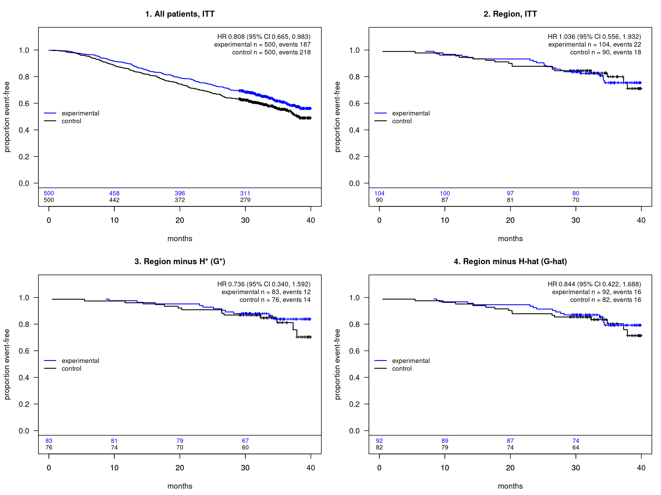
All patients, ITT	1000	500 / 187	500 / 218	0.808	0.665, 0.983
Region, ITT	194	104 / 22	90 / 18	1.036	0.556, 1.932
Region minus H* (G*)	159	83 / 12	76 / 14	0.736	0.340, 1.592
Region minus Ĥ (Ĝ)	174	92 / 16	82 / 16	0.844	0.422, 1.688

mrct_four_sets() takes the trial’s columns and this membership of $\hat H$, and its plot() draws the forest plot and the Kaplan–Meier panels, by the code plot() uses for an mrct_case_study object (simulations article).

Code

sets4 <- mrct_four_sets(trial, "y_sim", "event_sim", "treat_sim", region.name = "z_region",
                        in_Hhat = in_Hhat, truth.name = "flag_harm")
plot(sets4, which = "forest")

Figure 1: Replicate 5 of S2: hazard ratio, experimental vs control, with 95% CI (log scale).

Code

plot(sets4, which = "km", time_unit = "months", analysis_time = 40)

Replicate 5 of S2: Kaplan–Meier by arm in the four sets (experimental blue, control black; months).

The trial is positive (ITT upper limit 0.983 < 1.0) and its region is above 1.0 (1.036, 40 events): the trigger. Applied in the region, $\hat H$ removes 20 patients, and region($\hat G$) is 0.844, below 1.0: the trial is joint. Every interval is wide: the regional sets have few events, so the move of the regional estimate from above 1 to below 1 is an explanation consistent with a trial-wide harmed subgroup, not confirmation of it. With your trial: fs_in_subgroup() applies your $\hat H$ to all your rows; without truth.name, mrct_four_sets() drops the region($G^*$) row, as $H^*$ is unknown.

What the move below 1.0 shows, and what it does not

Removing $\hat H$ from the region and refitting the Cox model compares two different patient sets; it does not decompose the regional hazard ratio. The region’s estimate is not a weighted average of the estimates in $\hat H$ and in $\hat G$: removing patients changes the risk sets, the events and the censoring mixture, and each Cox estimate converges to the limit of its own set at the analysis time (appendix), which can differ from that set’s AHR or CDE. A regional estimate that moves from above 1.0 to below 1.0 is therefore compatible with a trial-wide subgroup accounting for the regional result. It does not show that $\hat H$ caused it, does not validate $\hat H$ as a clinically actionable subgroup, and, read with the null cells of the simulations article, can arise when there is no harmed subgroup at all. Nor is the distance between region($\hat G$) and region($G^*$) a measure of how well $\hat H$ recovered $H^*$: they are different patient sets, and each estimate converges to its own set’s limit (the simulations article sets $\hat H$ against $H^*$ directly).

2.5 Step 5: the Pareto frontier and the bounds

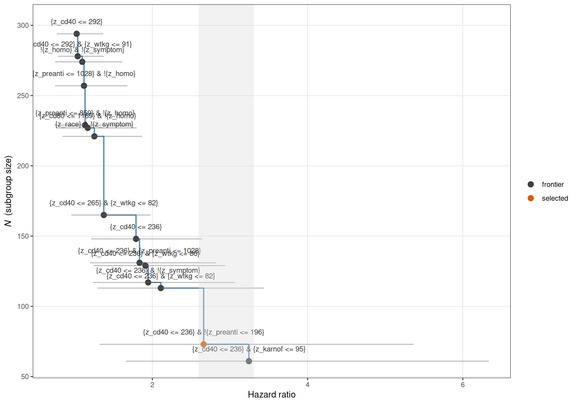
The Pareto frontier: the admitted candidates that no other candidate beats on both hazard ratio and size, with half-sample (split) 95% intervals from compute_frontier_cis() (1,000 random halvings per member) and the effect neighbourhood 0.20 shaded; $\hat H$ is the selected member.

Code

ci_front <- compute_frontier_cis(fs, n_splits = 1000L, seed = seed_rep5)
pf <- fs$grp.consistency$out_sg$pareto_frontier
stopifnot(nrow(ci_front) == nrow(pf), sum(pf$N == mr$n_selected & abs(pf$hr - mr$naive$est) < 1e-6) == 1)
print(plot_pareto_frontier(fs, ci_table = ci_front, show_band = TRUE, effect_neighborhood = 0.20))

The inference table, by mr_estimates_table() from the forestsearch() result alone. Two sets are bounded, both among the non-region patients: $\hat H$ (row Qstnbl) and $\hat H^c$, its non-region complement (row Recmnd). $\hat H^c$ is not $\hat G$; the region’s outcomes play no part.

Code

mr_tab <- mr_estimates_table(fs, est.scale = "hr", digits = 3)
mv <- attr(mr_tab, "mr_values")
cc <- mr$complement; fl <- mr$field
stopifnot(near(mv$naive_est, c(mr$naive$est, cc$naive$est), 1e-12),
          near(mv$field_bound, c(fl$lower_1s, fl$complement$upper_1s), 1e-12),
          near(mv$bonferroni_bound, c(fl$joint$bonf_lower_H, fl$joint$bonf_upper_Hc), 1e-12))
mr_tab

Treatment Effect by Subgroup
Naive and multiplier-resampling (MR) estimates (2000 draws)
Subgroup	Sample Size			Survival			Treatment Effect	Multiplier resampling (MR)1
	N	NT	Events	MedT	MedC	RMSTd	HR (95% CI, robust)†2	De-biased (95% IJ CI)	Field one-sided 95%	Bonferroni pair (joint 95%)
Qstnbl3	73 (9.1%)	36 (49.3%)	67 (91.8%)	10.1	19.7	-8	2.661 (1.482, 4.780)	1.629 (0.816, 3.249)	≥ 0.850	≥ 0.720
Recmnd	733 (90.9%)	360 (49.1%)	298 (40.7%)	NA	37.5	2.9	0.725 (0.577, 0.910)	0.753 (0.482, 1.175)	≤ 0.904	≤ 0.930
1 MR: the selected estimate de-biased for its selection over the re-selections of multiplier draws within the fixed candidate family; two-sided infinitesimal-jackknife (IJ) interval; field: one-sided 95% bound from the nested Monte Carlo of the re-selection (lower for the selected subgroup, upper for its complement on the HR scale); Bonferroni pair: the two bounds each at 97.5%, jointly 95%.
2 Unadjusted HR: Standard Cox regression hazard ratio with robust standard errors
3 Identified subgroup: {z_cd40 <= 236} & !{z_preanti <= 196}
Note: Med = Median survival time (months). RMSTd = Restricted mean survival time difference.

Read by location: the naive hazard ratio of $\hat H$ is 2.661 and its de-biased value 1.629, but the field lower bound is 0.850, below 0.90: once the selection is accounted for, the data do not rule out a modest benefit in $\hat H$ — and a lower bound does not establish harm there either. The field upper bound for $\hat H^c$ is 0.904, below 1.0: the non-region patients outside $\hat H$ benefit. The two bounds are one-sided statements about two different sets, not an interval for the contrast between them, so together they do not establish that the two effects are separated; the Bonferroni pair in the table is the joint statement. $\hat H$ is re-selected on a share 0.186 of the draws. With your trial: nothing changes; compute_frontier_cis() and mr_estimates_table() take your forestsearch() result.

Reading the bounds

mr_estimates_table() needs only the forestsearch() result run with mr_inference = TRUE. Read the field lower bound for $\hat H$ by its location against the hazard ratios that would matter clinically in your setting: a lower bound well below 1.0 leaves benefit in $\hat H$ open; one near or above 0.90 says that, after accounting for the selection, little benefit remains there. Read the field upper bound for $\hat H^c$ the same way: below 1.0 says the non-region patients outside $\hat H$ benefit. Use the Bonferroni pair when both statements are made together. The naive estimate in $\hat H$ is selected and is not a bound. The field bounds are not ordinary intervals computed after treating $\hat H$ as fixed: they are selection-adjusted by construction, bounds over the multiplier draws of the whole candidate family. The re-selection share $\hat p(\hat H)$ is a stability diagnostic for the exact declared rule: a small share says another rule would often have been declared from similar data. It does not say whether neighbouring rules or the broader patient pattern are stable, and it is not evidence for or against a harmed subgroup existing.

These bounds are for sets among the non-region patients. The region’s fits on the whole region and on $\hat G$ are ordinary Wald fits on sets defined by a fixed rule, with the region’s few events; read their intervals by location as well.

Because replicate 5 is simulated, its $\hat H$ can also be set against $H^*$ and its estimates against their limits; that needs the simulation design, and is in the simulations article.

2.6 The S2 campaign in brief

Replicate 5 is one trial of S2. The campaign ran 10,000 trials of the same design (the simulations article). The first table gives the campaign-observed counterparts of the analytic rows of Section 1.3 — unconditional, over all trials; the second follows the pipeline of this section, conditional on the trigger where its denominators say so. The numbers are read from the campaign’s records, shipped with the package.

Code

cc_core <- mrct_record("core_full_numeric.csv")
cc_core <- cc_core[cc_core$setting == "S2_rmlog4", ]
cc_disp <- mrct_record("core_n1000.csv")
stopifnot(nrow(cc_core) == 1, cc_core$replicates == 10000)
# the trial-positive count, from the display record's first row for S2 ("...; N of M)")
r1 <- cc_disp$value[cc_disp$row == "r1" & cc_disp$column == "S2"]
n_A <- as.numeric(gsub(",", "", sub("^.*; ([0-9,]+) of [0-9,]+\\)$", "\\1", r1)))
reps <- cc_core$replicates
n_trig <- cc_core$n_trigger
n_orac <- cc_core$n_Gstar_lt1
n_dcl  <- cc_core$n_declared_Ghat_lt1
stopifnot(length(n_A) == 1, !is.na(n_A), n_trig <= n_A, n_orac <= n_trig, n_dcl <= n_trig)
# row (2), over all trials: the entry-cells record's S2 column is this campaign (three shared counts checked)
cc_ent <- mrct_record("entry_cells_core_numeric.csv")
cc_ev <- function(q) cc_ent$S2[cc_ent$quantity == q]
n_B <- round(cc_ev("p_region_itt_gt1") * reps)
stopifnot(cc_ev("n_trials") == reps, near(cc_ev("p_region_itt_gt1") * reps, n_B), n_trig <= n_B,
          near(c(cc_ev("p_itt_ub_lt1"), cc_ev("p_trigger"), cc_ev("p_trigger_Gstar_lt1")) * reps,
               c(n_A, n_trig, n_orac)))
counts <- c(n_A, n_A - n_trig, n_trig, n_orac, n_trig - n_orac,
            (n_A - n_trig) + n_orac, n_dcl, (n_A - n_trig) + n_dcl)
obs <- counts / reps
# identities by construction: (3)+(4)=(1), (5)+(6)=(4), (3)+(5)=(7), (3)+(8)=(9)
stopifnot(near(obs[2] + obs[3], obs[1], 1e-12), near(obs[4] + obs[5], obs[3], 1e-12),
          near(obs[2] + obs[4], obs[6], 1e-12), near(obs[2] + obs[7], obs[8], 1e-12))
lab_obs <- c("(1) P(ITT ub < 1.0): the trial is positive",
             "(3) P(consistency): positive, region ITT ≤ 1.0",
             "(4) P(non-consistency): the trigger",
             "(5) P(oracle consistency): the oracle joint",
             "(6) P(oracle non-consistency)",
             "(7) P(consistency or oracle consistency)",
             "(8) P̂(declared consistency)",
             "(9) P̂(consistency or declared consistency)")
knitr::kable(data.frame(row = append(lab_obs, "(2) P(region ITT > 1.0)", after = 1),
                        `campaign-observed` = append(sprintf("%s (%s)", f3(obs), big(counts)),
                                                     sprintf("%s (%s)", f3(n_B / reps), big(n_B)), after = 1),
                        check.names = FALSE),
             row.names = FALSE, align = "lr",
             caption = "S2 at n = 1,000, campaign-observed over 10,000 trials; rows as in @sec-predictions, identities asserted.")

S2 at n = 1,000, campaign-observed over 10,000 trials; rows as in Section 1.3, identities asserted.

row	campaign-observed
(1) P(ITT ub < 1.0): the trial is positive	0.840 (8,397)
(2) P(region ITT > 1.0)	0.327 (3,266)
(3) P(consistency): positive, region ITT ≤ 1.0	0.600 (5,999)
(4) P(non-consistency): the trigger	0.240 (2,398)
(5) P(oracle consistency): the oracle joint	0.186 (1,864)
(6) P(oracle non-consistency)	0.053 (534)
(7) P(consistency or oracle consistency)	0.786 (7,863)
(8) P̂(declared consistency)	0.123 (1,228)
(9) P̂(consistency or declared consistency)	0.723 (7,227)

Code

cc_mr <- mrct_record("mr_field_core.csv")
stopifnot(sum(cc_mr$row == "lb_100") == 1,
          sum(cc_ent$quantity %in% c("trigger_n", "joint", "Ghat_region")) == 3)
camp <- list(
  reps = reps, n_trig = n_trig, n_decl = cc_core$n_declared, n_joint = n_dcl,
  lb100 = as.numeric(cc_mr$S2[cc_mr$row == "lb_100"]),
  ghat_reg = cc_ev("Ghat_region"))
camp$p_trig <- 100 * camp$n_trig / camp$reps
camp$p_decl <- 100 * camp$n_decl / camp$n_trig
camp$p_joint <- 100 * camp$n_joint / camp$n_trig
# the two records agree on S2
stopifnot(camp$n_trig == cc_ev("trigger_n"), abs(camp$p_joint - cc_ev("joint")) <= 1e-9)
# the reading's verbal claims
stopifnot(round(camp$p_trig / 25) == 1, abs(camp$p_joint - 50) < 5)
pc1 <- function(x) formatC(x, format = "f", digits = 1)
knitr::kable(
  data.frame(
    step = c("trigger: ITT ub < 1.0 and region ITT > 1.0", "subgroup declared",
             "Ĥ field lower bound (one-sided 95%) > 1.0", "declared, region(Ĝ) < 1.0",
             "Ĝ, % of region patients"),
    S2 = c(sprintf("%s (%s)", pc1(camp$p_trig), big(camp$n_trig)),
           sprintf("%s (%s)", formatC(camp$p_decl, format = "f", digits = 2), big(camp$n_decl)),
           pc1(camp$lb100),
           sprintf("%s (%s)", pc1(camp$p_joint), big(camp$n_joint)),
           pc1(camp$ghat_reg)),
    of = c(sprintf("all trials (%s)", big(camp$reps)), "triggered trials", "declared triggered trials",
           "triggered trials", "declared triggered trials")),
  align = "lrl",
  caption = "Conditional on the trigger: the pipeline of this section, as often as it went each way (each row's denominator stated).")

Conditional on the trigger: the pipeline of this section, as often as it went each way (each row’s denominator stated).

step	S2	of
trigger: ITT ub < 1.0 and region ITT > 1.0	24.0 (2,398)	all trials (10,000)
subgroup declared	99.96 (2,397)	triggered trials
Ĥ field lower bound (one-sided 95%) > 1.0	13.6	declared triggered trials
declared, region(Ĝ) < 1.0	51.2 (1,228)	triggered trials
Ĝ, % of region patients	87.2	declared triggered trials

Read unconditionally: the trial is positive in 0.840 of trials; consistency holds outright in 0.600, and the trigger occurs in 0.240 — about one S2 trial in four. The oracle resolution holds in 0.186 of all trials (row 5) and the declared subgroup’s in 0.123 (row 8), so the two routes together give 0.786 by the oracle pathway and 0.723 by the declared pathway (rows 7 and 9). Conditional on the trigger: a subgroup was declared in 2,397 of 2,398 triggered trials, region(Ĝ) was below 1.0 in about half (51.2%), and Ĝ kept on average 87.2% of the region’s patients. The field lower bound for Ĥ was above 1.0 in 13.6% of the declared triggered trials; in the others it lies below 1.0, and it is read by its location, as for replicate 5 in step 5. Replicate 5 is one of the triggered trials with region(Ĝ) < 1.0.

2.7 The one-call form

mrct_trial_analysis() is steps 1 to 5 in one call: the two Cox fits and the trigger, the identifier on the non-region patients with multiplier resampling, $\hat H$ applied to every row, and the four sets. Here it runs on the same trial, with the identifier’s arguments of step 3 and the record’s seed.

Code

one_call <- mrct_trial_analysis(
  trial, "y_sim", "event_sim", "treat_sim", region.name = "z_region", id.name = "id",
  truth.name = "flag_harm",
  fs_args = list(confounders.name = covs, conf_force = character(0),
                 conf.cont_jcuts = list(z_cd40 = 10, z_wtkg = 10, z_preanti = 10),
                 use_grf = FALSE, use_lasso = FALSE, maxk = 2,
                 hr.threshold = 0.90, hr.consistency = 0.80, pconsistency.threshold = 0.90,
                 sg_focus = "hrMaxSG", effect_neighborhood = 0.20),
  mr_inference_args = list(ci_method = "field", include_complement = TRUE, field_complement = TRUE,
                           draws = 2000, multiplier = "poisson", return_reselection = TRUE,
                           seed = seed_rep5))
one_call

MRCT trial analysis: n = 1000, region 'z_region'
Stage: complete
H-hat: {z_cd40 <= 236} & !{z_preanti <= 196}
Trigger (ITT ub < 1.0 and region ITT > 1.0): TRUE

 Set                        n    exp n/events ctl n/events HR    95% CI
 All patients, ITT          1000 500/187      500/218      0.808 0.665, 0.983
 Region, ITT                 194 104/22       90/18        1.036 0.556, 1.932
 Region minus H* (G*)        159 83/12        76/14        0.736 0.340, 1.592
 Region minus H-hat (G-hat)  174 92/16        82/16        0.844 0.422, 1.688

H-hat against H* (TP, FP, FN, TN):
  nonregion  65, 8, 65, 668
  region     18, 2, 17, 157

Multiplier resampling (field, 2000 draws):
 set                           naive debiased IJ 95% CI    field 1-sided 95%
 H-hat                         2.661 1.629    0.816, 3.249 >= 0.850
 H-hat complement (non-region) 0.725 0.753    0.482, 1.175 <= 0.904
 field-s 1-sided 95% Bonferroni Bonferroni, field-s
 -                   >= 0.720   >= 0.720
 <= 0.908            <= 0.930   <= 0.933           

Code

# its H-hat, four sets and MR values equal the step-by-step objects above
num <- c("n", "n_exp", "n_ctl", "events_exp", "events_ctl", "hr", "lo", "hi")
mv_call <- mr_values(one_call$fs); mv_step <- mr_values(fs)
keep <- !grepl("timing", names(mv_step))
stopifnot(identical(one_call$Hhat, Hhat_def), identical(one_call$in_Hhat, in_Hhat),
          identical(one_call$sets$set, four$set),
          isTRUE(all.equal(one_call$sets[num], four[num], tolerance = 1e-12)),
          isTRUE(all.equal(mv_call[keep], mv_step[keep], tolerance = 1e-12)))

With your trial: your column names, your covariates in fs_args$confounders.name and your seed in mr_inference_args, without truth.name. $stage says how far the pipeline went (not_positive, no_trigger, no_declaration or complete), and none of these is an error; plot() on the result draws the two figures of step 4, and mr_values() and mr_estimates_table() read its $fs.

The article took 3.2 minutes to run.

Appendix: the analysis window and the windowed Cox limit

This appendix works through the callout “The windowed Cox limit” of Section 1.2 for S2, on the build of Section 1.3 (dgm_pre, whose hazard scale and regional shift are estimated from replicate 5).

What the multiplier changes. scale_dgm_hazard(dgm, m) replaces the intercept $\mu$ by $\mu - \tau\log m$, so $\Lambda_0(s) = (s\,e^{-\mu})^{1/\tau}$ becomes $$m\,\Lambda_0(s) = \Lambda_0(m^{\tau} s):$$ every patient’s hazard, on both arms, is multiplied by $m$, which is the same as running every patient’s clock $m^{\tau}$ times faster. No $\theta_z(X)$ changes, so no patient’s hazard ratio changes, and neither do three summaries of a set that depend on the $\theta$’s alone: the AHR, the CDE, and margHR($\infty$) — a Cox fit with no censoring uses only the order of the event times, and running every clock faster does not reorder them. What changes is how many events fall inside the analysis window, whose limits are fixed in calendar months.

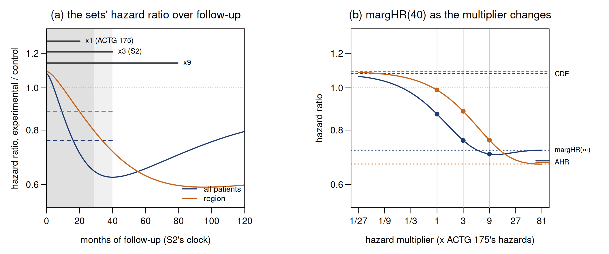
A set’s hazard ratio over follow-up. At month $s$ of follow-up, a set’s hazard ratio is each arm’s mean hazard among its patients still event-free, experimental over control. At $s = 0$ every patient is at risk and it is the CDE; then it moves as patients have events (Figure 2, panel a). In S2 both the trial’s and the region’s start above 1.0 and fall below it within the first year.

What the Cox fit estimates. margHR(40) is the constant hazard ratio that, applied to the patients at risk at every event time, reproduces the experimental arm’s share of the events inside the window: in effect, an average of the set’s curve over the window’s events. In panel (a) the window is shaded (every patient is followed to 29 months, the last enrolled to 40) and the dashed segments are the two sets’ margHR(40).

Code

# dgm_pre runs on S2's clock (x 3, estimated from the trial): scaling it by M / 3 puts it at M x ACTG 175's hazards
M_grid <- 3^seq(-3, 4, by = 0.25)
clock <- do.call(rbind, lapply(M_grid, function(M) {
  pop_M <- ahr_population(scale_dgm_hazard(dgm_pre, M / 3), analysis_time = 40, max_entry = 11)
  do.call(rbind, lapply(c("all", "region"), function(s) {
    e <- ahr_limit(pop_M, s, b = 0.55, h = 2, variance = FALSE)
    data.frame(M = M, set = s, margHR40 = e$hr, AHR = e$ahr, CDE = e$cde,
               margHRinf = e$marghr_inf, events = e$d)
  }))
}))
ck <- function(s, M, v) clock[[v]][clock$set == s & abs(clock$M - M) < 1e-9]
# the region without its prognostic shift, at S2's rate: S2 with every hazard multiplied by exp(-r)
pop_nor <- ahr_population(scale_dgm_hazard(dgm_pre, exp(-r_pre)), analysis_time = 40, max_entry = 11)
reg_nor <- ahr_limit(pop_nor, "region", b = 0.55, h = 2, variance = FALSE)$hr
# a set's hazard ratio at month s: each arm's mean hazard among its event-free patients
hr_at <- function(dgm, in_set, months) {
  ds <- dgm$df_super[in_set, ]; mp <- dgm$model_params
  e0 <- exp(ds$theta_0); e1 <- exp(ds$theta_1)
  vapply(months, function(s) {
    u <- (s * exp(-mp$mu))^(1 / mp$tau)                  # Lambda_0(s), S2's clock
    (sum(e1 * exp(-u * e1)) / sum(exp(-u * e1))) / (sum(e0 * exp(-u * e0)) / sum(exp(-u * e0)))
  }, numeric(1))
}
months <- seq(0, 120, by = 0.5)
in_reg <- dgm_pre$df_super$z_region == 1
prof <- list(all = hr_at(dgm_pre, rep(TRUE, length(in_reg)), months), region = hr_at(dgm_pre, in_reg, months))
tau <- dgm_pre$model_params$tau
reach <- 40 * (c(1, 3, 9) / 3)^tau                         # where 40 months at x1, x3, x9 end on S2's clock
# the multiplier leaves each set's AHR, CDE and margHR(inf) unchanged; each curve starts at its CDE
for (s in c("all", "region")) for (v in c("AHR", "CDE", "margHRinf"))
  stopifnot(near(clock[[v]][clock$set == s], ck(s, 3, v), 1e-6))
stopifnot(near(c(prof$all[1], prof$region[1]), c(ck("all", 3, "CDE"), ck("region", 3, "CDE")), 1e-9))
# the verbal claims of this appendix and of the callout in the design section
stopifnot(all(vapply(prof, function(p) p[1] > 1 && min(p[months <= 12]) < 1, NA)),
          abs(ck("all", 1/27, "margHR40") / ck("all", 3, "CDE") - 1) < 0.02,
          abs(ck("all", 81, "margHR40") / ck("all", 3, "margHRinf") - 1) < 0.002,
          abs(log(ck("all", 3, "AHR") / c(ck("all", 3, "CDE"), ck("all", 3, "margHRinf")))) > 0.01,
          ck("region", 3, "margHR40") / ck("region", 3, "CDE") > ck("all", 3, "margHR40") / ck("all", 3, "CDE"),
          ck("region", 3, "margHR40") > ck("all", 3, "margHR40"), reg_nor < ck("all", 3, "margHR40"),
          round(5 * ck("all", 1, "events")) == 1)

Code

col_set <- c(all = "#1f3b73", region = "#c4661f")
op <- par(mfrow = c(1, 2), mar = c(4.2, 4.2, 2.6, 5.4), mgp = c(2.4, 0.7, 0), las = 1)
# (a) each set's hazard ratio over follow-up
plot(NA, xlim = c(0, 120), ylim = c(0.55, 1.32), log = "y", xaxs = "i",
     xlab = "months of follow-up (S2's clock)", ylab = "hazard ratio, experimental / control",
     main = "(a) the sets' hazard ratio over follow-up", font.main = 1)
rect(0, 0.5, 29, 1.4, col = "grey88", border = NA); rect(29, 0.5, 40, 1.4, col = "grey94", border = NA)
abline(h = 1, col = "grey50", lty = 3)
for (s in names(prof)) {
  lines(months, prof[[s]], col = col_set[[s]], lwd = 2)
  segments(0, ck(s, 3, "margHR40"), 40, ck(s, 3, "margHR40"), col = col_set[[s]], lty = 2, lwd = 1.5)
}
y_bar <- c(1.28, 1.21, 1.14)
segments(0, y_bar, reach, y_bar, lwd = 2.5, col = "grey25")
text(reach, y_bar, c("x1 (ACTG 175)", "x3 (S2)", "x9"), pos = 4, cex = 0.8)
legend("bottomright", c("all patients", "region"), col = col_set, lwd = 2, bty = "n", cex = 0.85)
box()
# (b) margHR(40) against the hazard multiplier
plot(NA, xlim = range(clock$M), ylim = c(0.55, 1.32), log = "xy", xaxt = "n",
     xlab = "hazard multiplier (x ACTG 175's hazards)", ylab = "hazard ratio",
     main = "(b) margHR(40) as the multiplier changes", font.main = 1)
axis(1, at = 3^(-3:4), labels = c("1/27", "1/9", "1/3", "1", "3", "9", "27", "81"))
abline(v = c(1, 3, 9), col = "grey80"); abline(h = 1, col = "grey50", lty = 3)
for (s in c("all", "region")) {
  d <- clock[clock$set == s, ]
  abline(h = d$CDE[1], col = col_set[[s]], lty = 2)
  abline(h = d$margHRinf[1], col = col_set[[s]], lty = 3, lwd = 1.5)
  axis(4, at = d$AHR[1], labels = FALSE, col.ticks = col_set[[s]], lwd.ticks = 2, tcl = 1.2)
  lines(d$M, d$margHR40, col = col_set[[s]], lwd = 2)
  keep <- d$M %in% c(1, 3, 9)
  points(d$M[keep], d$margHR40[keep], pch = 19, col = col_set[[s]])
}
mtext(c("CDE", expression("margHR(" * infinity * ")"), "AHR"), side = 4, line = 0.5, las = 1,
      cex = 0.75,
      at = c(ck("all", 3, "CDE"), ck("all", 3, "margHRinf"), mean(c(ck("all", 3, "AHR"), ck("region", 3, "AHR")))))
par(op)

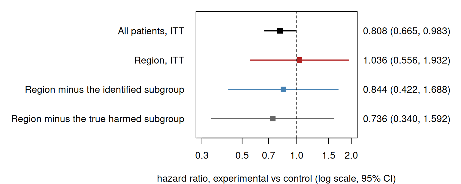
Figure 2: S2, as built in Section 1.3. (a) Each set’s hazard ratio at each month of follow-up on S2’s clock (each arm’s mean hazard among the set’s event-free patients); shaded, the 40-month analysis window; dashed, each set’s margHR(40); bars, how far 40 months reach on this clock at 1, 3 and 9 times ACTG 175’s hazards. (b) margHR(40) against the hazard multiplier, with each set’s CDE (dashed) and margHR(∞) (dotted); the right-hand ticks are the AHRs.

The window sits later on the faster clock. By $m\,\Lambda_0(s) = \Lambda_0(m^{\tau} s)$, a trial at $m$ times the hazards, analysed at 40 months, sees what the unscaled trial sees at $40\,m^{\tau}$ months, with its entry period stretched alike: the curves stay where they are, and the fixed 40-month window covers more of them. With $\hat\tau$ = 0.624, 40 months at ACTG 175’s rate (×1) cover the first 20 months of S2’s clock, and at ×9 the first 79 (the bars in panel a). Panel (b) follows margHR(40) across multipliers. As $m \to 0$ the few events come before anyone has left, and the limit tends to the CDE; as $m \to \infty$ every event falls inside the window, and it tends to margHR($\infty$). In between it moves although no patient’s hazard ratio has: for all patients from 0.871 at ×1 to 0.757 at S2’s ×3, and for the region from 0.989 to 0.884, while the share of patients with an event in the window goes from 18.3% to 39.0%. Neither end is the AHR (0.680 for all patients).

The region runs on a slower clock. The shift $r$ multiplies the region’s hazards by $e^{r}$ on both arms, so it acts on the region exactly as a multiplier acts on the trial: the region with its shift, at multiplier $m$, is the region without it at $m\,e^{r}$. Here $e^{\hat r}$ = 0.214 slows the region’s clock: its curve in panel (a) runs later, and its 40-month window ends earlier on it, nearer the CDE. Removing the shift — for the region’s own limit, the same as multiplying every hazard by $e^{-\hat r}$, one more scale_dgm_hazard() call — moves the region’s margHR(40) at S2’s rate from 0.884 to 0.719, below the trial’s 0.757.

What follows.

• The multiplier sets the event rate and nothing else: $b$, $h$, and every set’s AHR, CDE and margHR($\infty$) are as set at every multiplier.
• The pipeline’s Cox fits estimate their sets’ margHR(40), so where the trial’s estimates fall — and with them the probabilities of Section 1.3 — depends on the event rate and the window as well as on the effects. A regional estimate near or above 1.0 can come from a trial-wide harmed subgroup in a region of lower baseline risk, with no regional difference in treatment effect: the region’s window holds the early part of its curve, where the harmed patients’ events weigh most.
• In a real trial nothing is multiplied: the trial’s own event rate and follow-up set the clock. The same set can give a different Cox estimate at a later analysis with no patient’s effect changed, and a region of lower baseline risk is seen earlier on its curve than the rest of the trial at the same analysis time.

Appendix: the manuscript’s event notation

The accompanying manuscript collects the design’s events in its Table 1, reproduced here; a superscript $+$ ($-$) marks a point estimate or bound in (opposite to) the direction of consistency. This article’s $A$, $B$ and $C^*$ are $\mathrm{ITT}^+$, $\mathrm{R}^-$ and $\mathrm{R}(G^*)^+$.

The manuscript’s Table 1: event notation.

Event	Definition	Reading
Primitive events
$\mathrm{ITT}^+$	{ITT 95% upper bound < 1.0}	The trial is positive
$\mathrm{R}^-$, $\mathrm{R}^+$	{region ITT > 1.0}, {region ITT $\le$ 1.0}	Region point estimate opposite to, in, the direction of consistency
$\mathrm{R}(G^*)^-$, $\mathrm{R}(G^*)^+$	{region($G^*$) > 1.0}, {region($G^*$) $\le$ 1.0}	Likewise, for the region outside the true subgroup $H^*$
$\mathrm{R}(\hat G)^+$	{subgroup declared, region($\hat G$) < 1.0}	The declared resolution is in the consistent direction
Named events
consistency	$\mathrm{ITT}^+ \cap \mathrm{R}^+$	Positive trial, region in the consistent direction — the standard pathway
non-consistency	$\mathrm{ITT}^+ \cap \mathrm{R}^-$	Positive trial, region opposite — the trigger for subgroup identification
oracle consistency	$\mathrm{ITT}^+ \cap \mathrm{R}^- \cap \mathrm{R}(G^*)^+$	Non-consistency resolved by the true subgroup
oracle non-consistency	$\mathrm{ITT}^+ \cap \mathrm{R}^- \cap \mathrm{R}(G^*)^-$	Non-consistency persisting under the oracle resolution
declared consistency	$\mathrm{ITT}^+ \cap \mathrm{R}^- \cap \mathrm{R}(\hat G)^+$	Non-consistency resolved by the declared subgroup